pacman::p_load(treemap, treemapify, tidyverse, knitr)Chapter 16: Treemap Visualisation with R
Hands-on Exercise 5
16 Treemap Visualisation with R
16.1 Overview
A treemap displays hierarchical data as nested rectangles, where each rectangle’s area is proportional to a numeric measure and its colour can encode a second measure. This chapter covers static treemaps with the treemap package and treemapify, plus interactive treemaps with d3treeR.
16.2 Installing and Launching R Packages
Three packages are required:
- treemap for the foundational treemap implementation
- treemapify for
ggplot2-style treemap geoms - tidyverse for data wrangling
knitr is loaded so kable() can produce clean previews.
16.3 Data Wrangling
16.3.1 Importing the Data Set
The REALIS2018 dataset records private property transactions in Singapore, sourced from the URA REALIS portal. Each row is one transaction, which is too granular for a treemap, so aggregation is required.
realis2018 <- read_csv("data/realis2018.csv")16.3.2 Data Wrangling and Manipulation
The treemap requires aggregated values per leaf node in the hierarchy. The grouping is by Project Name, Planning Region, Planning Area, Property Type, and Type of Sale. The summary statistics are total units sold, total area, median unit price, and median transacted price.
16.3.3 Grouped Summaries Without the Pipe
The verbose two-step approach.
realis2018_grouped <- group_by(realis2018, `Project Name`,
                               `Planning Region`, `Planning Area`,
                               `Property Type`, `Type of Sale`)

realis2018_summarised <- summarise(realis2018_grouped,
                          `Total Unit Sold` = sum(`No. of Units`, na.rm = TRUE),
                          `Total Area` = sum(`Area (sqm)`, na.rm = TRUE),
                          `Median Unit Price ($ psm)` = median(`Unit Price ($ psm)`, na.rm = TRUE),
                          `Median Transacted Price` = median(`Transacted Price ($)`, na.rm = TRUE))
NoteThings to learn from the code chunk above
na.rm = TRUE is essential, because without it any missing value in any group would propagate to the summary and the corresponding rectangle would not render.
16.3.4 Grouped Summaries with the Pipe
The same logic, expressed more concisely.
realis2018_summarised <- realis2018 %>%
  group_by(`Project Name`, `Planning Region`,
           `Planning Area`, `Property Type`,
           `Type of Sale`) %>%
  summarise(`Total Unit Sold` = sum(`No. of Units`, na.rm = TRUE),
            `Total Area` = sum(`Area (sqm)`, na.rm = TRUE),
            `Median Unit Price ($ psm)` = median(`Unit Price ($ psm)`, na.rm = TRUE),
            `Median Transacted Price` = median(`Transacted Price ($)`, na.rm = TRUE))

kable(head(realis2018_summarised))| Project Name | Planning Region | Planning Area | Property Type | Type of Sale | Total Unit Sold | Total Area | Median Unit Price ($ psm) | Median Transacted Price |
|---|---|---|---|---|---|---|---|---|
| # 1 LOFT | Central Region | Geylang | Apartment | Resale | 1 | 51 | 13098.0 | 668000 |
| # 1 SUITES | Central Region | Geylang | Apartment | Resale | 1 | 52 | 12212.0 | 635000 |
| 1 CANBERRA | North Region | Yishun | Executive Condominium | Resale | 2 | 198 | 9056.5 | 896944 |
| 1 KING ALBERT PARK | Central Region | Bukit Timah | Condominium | Resale | 5 | 565 | 13986.0 | 1700000 |
| 10 EVELYN | Central Region | Novena | Apartment | New Sale | 2 | 96 | 26669.5 | 1280090 |
| 10 SHELFORD | Central Region | Bukit Timah | Apartment | Resale | 3 | 175 | 19714.0 | 833000 |
16.4 Designing Treemap with treemap Package
16.4.1 Designing a Static Treemap
First, filter to one segment to keep the visualisation readable. The example uses resale condominiums.
realis2018_selected <- realis2018_summarised %>%
  filter(`Property Type` == "Condominium",
         `Type of Sale` == "Resale")
16.4.2 Using the Basic Arguments
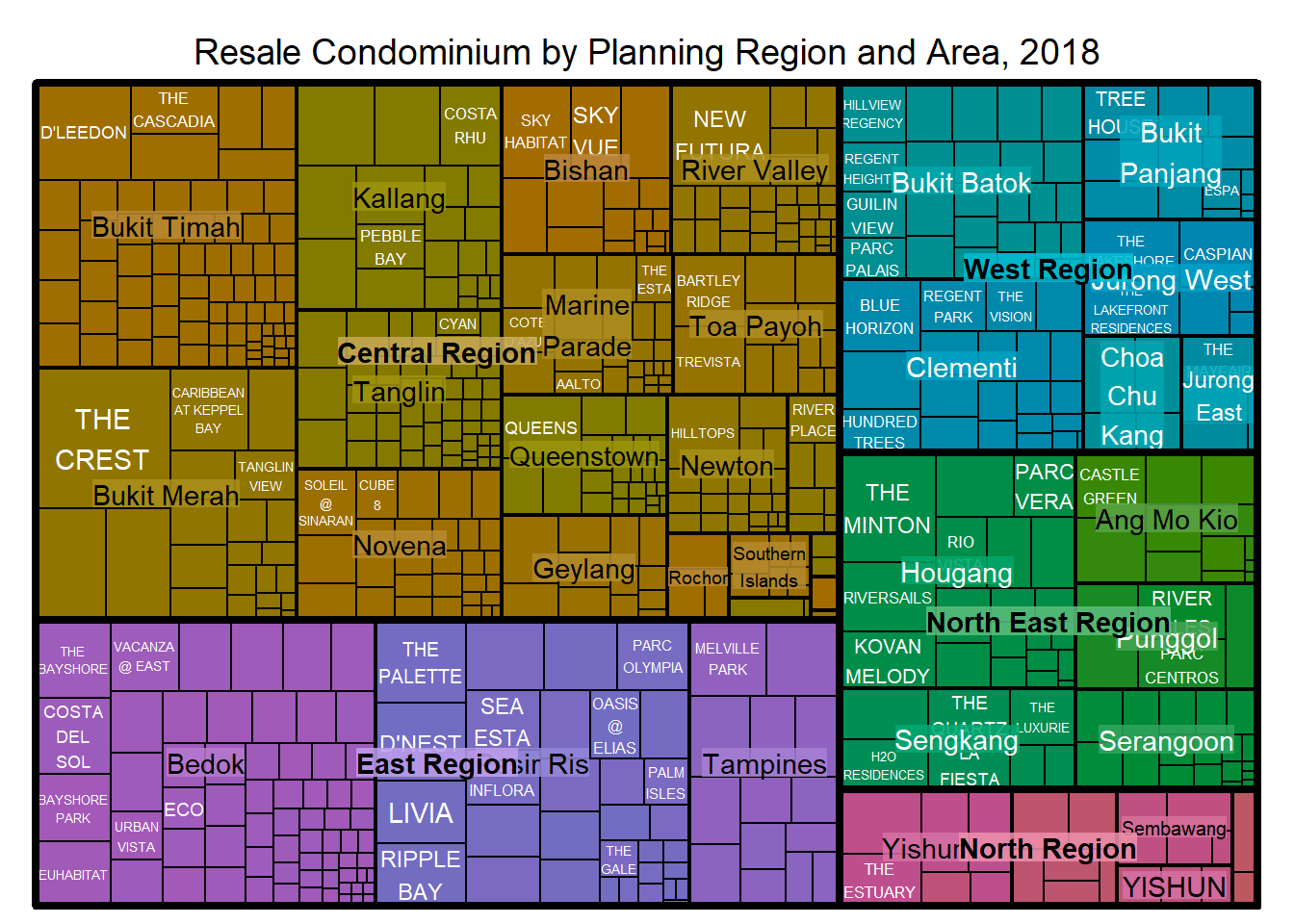
The minimal treemap requires three arguments: index (hierarchy), vSize (rectangle area), and vColor (rectangle colour).
treemap(realis2018_selected,
        index = c("Planning Region", "Planning Area", "Project Name"),
        vSize = "Total Unit Sold",
        vColor = "Median Unit Price ($ psm)",
        title = "Resale Condominium by Planning Region and Area, 2018",
        title.legend = "Median Unit Price (S$ per sq. m)")
ImportantCommon pitfall
The plot above is wrongly coloured. By default treemap() sets type = "index", which colours rectangles by the hierarchy level rather than by the vColor variable. The next section fixes this by setting type explicitly.
16.4.3 Working with vColor and type Arguments
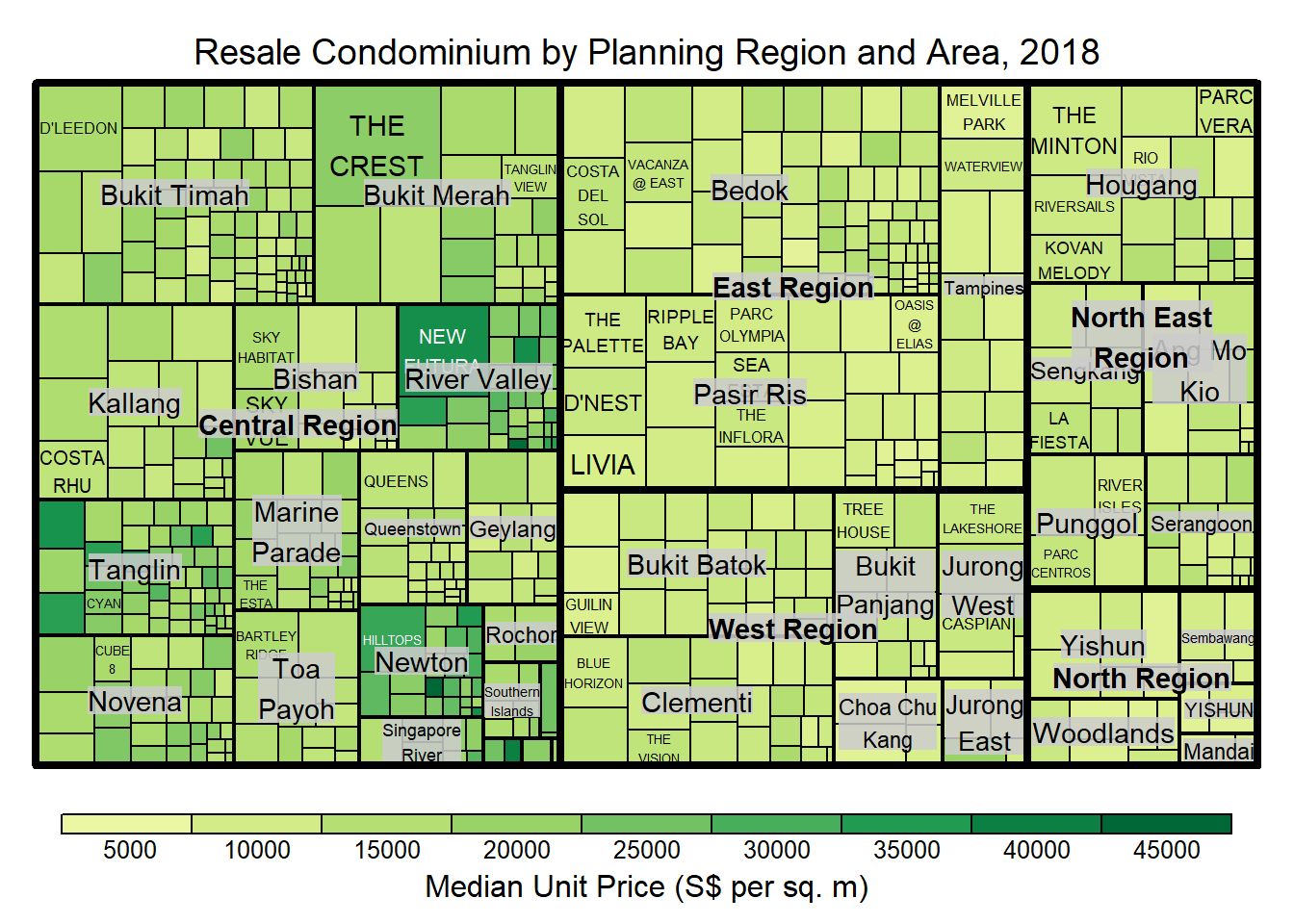
Setting type = "value" activates the diverging palette mapped from vColor.
treemap(realis2018_selected,
        index = c("Planning Region", "Planning Area", "Project Name"),
        vSize = "Total Unit Sold",
        vColor = "Median Unit Price ($ psm)",
        type = "value",
        title = "Resale Condominium by Planning Region and Area, 2018",
        title.legend = "Median Unit Price (S$ per sq. m)")
NoteThings to learn from the code chunk above
type = "value" interprets vColor as a continuous numeric variable and applies a divergent palette anchored at zero. The default binning is in equal intervals of 5,000 SGD per sq. m, visible in the legend.
16.4.4 Colours in treemap Package
Two arguments control the palette: mapping and palette. The value type centres the palette at zero with the maximum absolute value at the extremes. The manual type maps min, mean of range, and max linearly to the palette.
16.4.5 The “value” Type Treemap
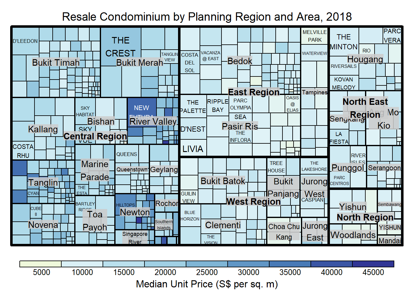
Using the RdYlBu palette with type = "value".
treemap(realis2018_selected,
        index = c("Planning Region", "Planning Area", "Project Name"),
        vSize = "Total Unit Sold",
        vColor = "Median Unit Price ($ psm)",
        type = "value",
        palette = "RdYlBu",
        title = "Resale Condominium by Planning Region and Area, 2018",
        title.legend = "Median Unit Price (S$ per sq. m)")
NoteThings to learn from the code chunk above
No red rectangles appear because all median unit prices are positive. The value type interprets the absence of negative values as the absence of one half of the palette.
16.4.6 The “manual” Type Treemap
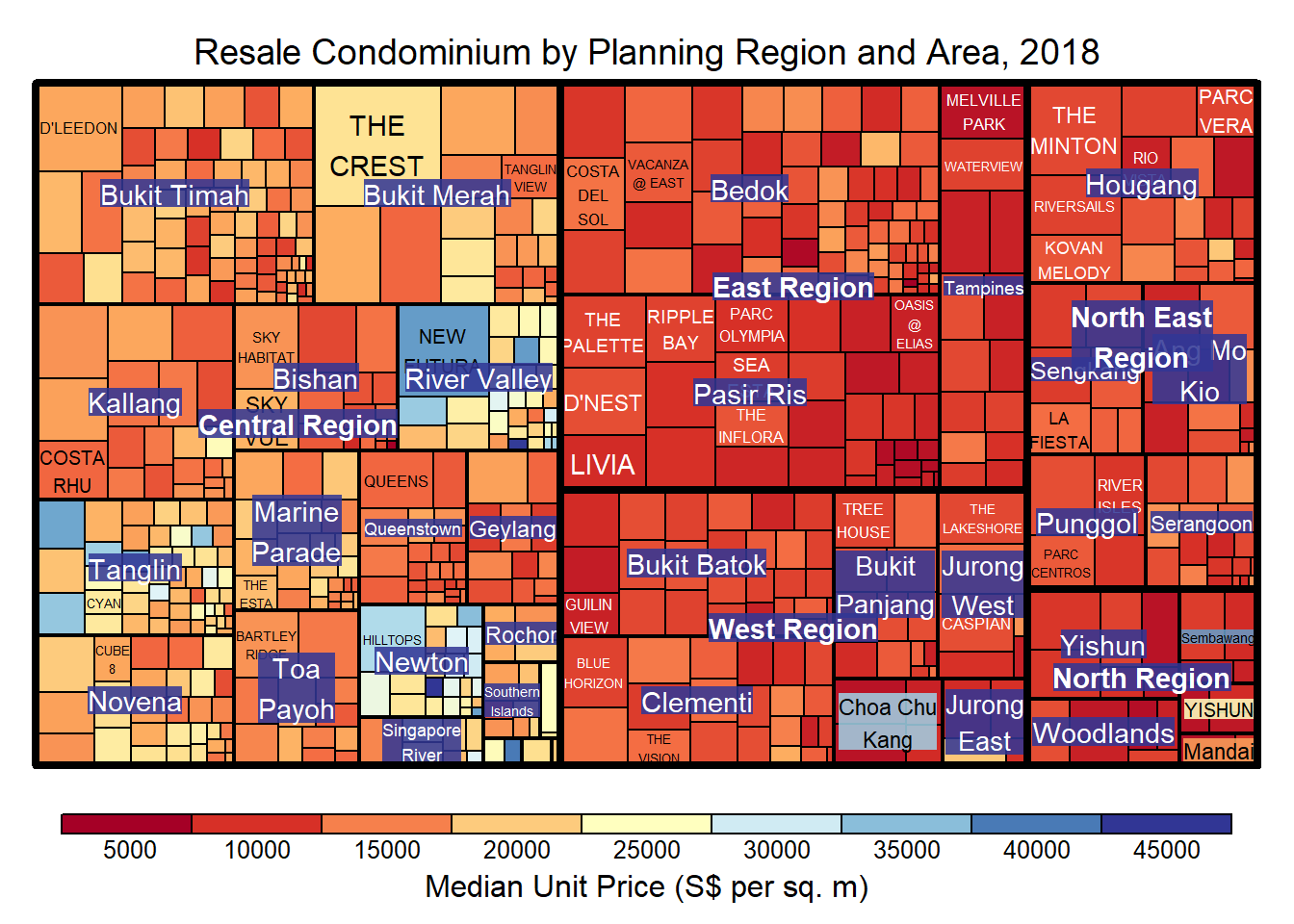
type = "manual" maps the actual min, mean, and max linearly to the palette.
treemap(realis2018_selected,
        index = c("Planning Region", "Planning Area", "Project Name"),
        vSize = "Total Unit Sold",
        vColor = "Median Unit Price ($ psm)",
        type = "manual",
        palette = "RdYlBu",
        title = "Resale Condominium by Planning Region and Area, 2018",
        title.legend = "Median Unit Price (S$ per sq. m)")
A sequential palette such as Blues is more appropriate for unipolar data.
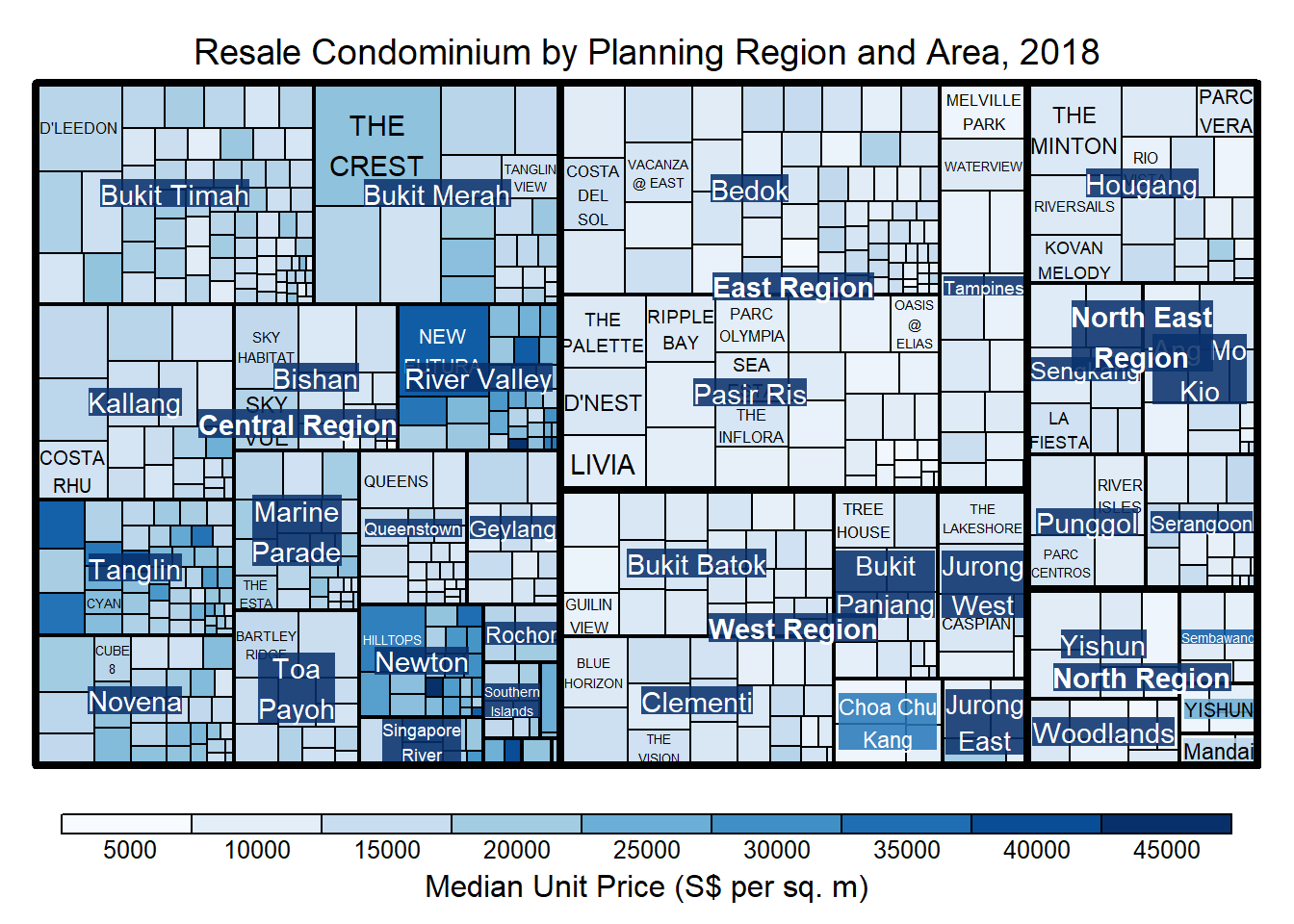
treemap(realis2018_selected,
        index = c("Planning Region", "Planning Area", "Project Name"),
        vSize = "Total Unit Sold",
        vColor = "Median Unit Price ($ psm)",
        type = "manual",
        palette = "Blues",
        title = "Resale Condominium by Planning Region and Area, 2018",
        title.legend = "Median Unit Price (S$ per sq. m)")
TipDiverging vs sequential palettes
The diverging palette implies that some prices are above some natural midpoint and some are below, which is misleading here because all prices are positive. The sequential palette conveys “more is darker” without implying a midpoint that does not exist.
16.4.7 Treemap Layout
treemap() supports two layout algorithms: "squarified", which optimises aspect ratios, and "pivotSize", the default, which respects sort order.
16.4.8 Working with algorithm Argument
The squarified layout produces nearly square rectangles.
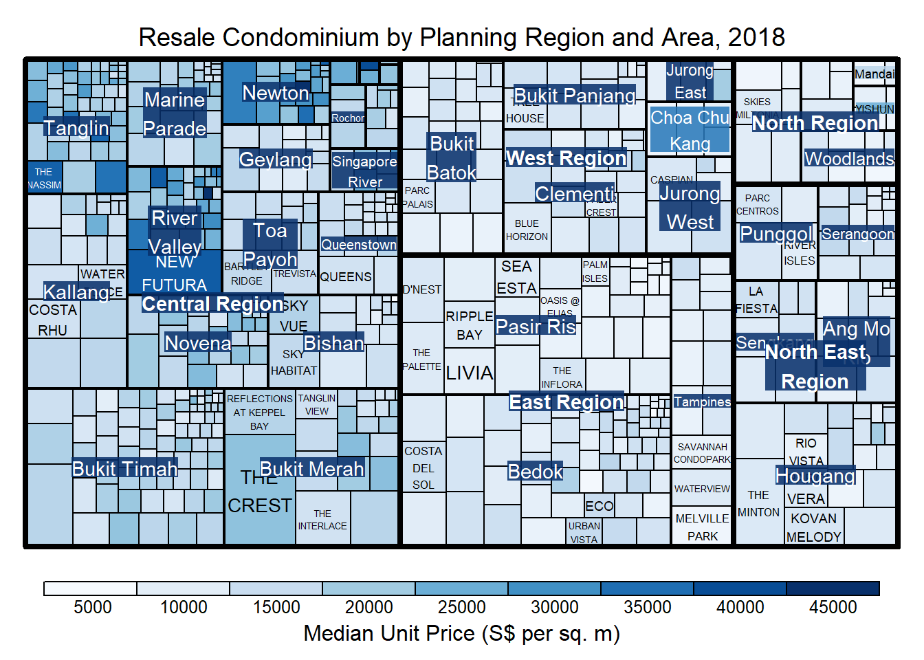
treemap(realis2018_selected,
        index = c("Planning Region", "Planning Area", "Project Name"),
        vSize = "Total Unit Sold",
        vColor = "Median Unit Price ($ psm)",
        type = "manual",
        palette = "Blues",
        algorithm = "squarified",
        title = "Resale Condominium by Planning Region and Area, 2018",
        title.legend = "Median Unit Price (S$ per sq. m)")
16.4.9 Using sortID
When algorithm = "pivotSize" is used, sortID controls the placement order from top-left to bottom-right.
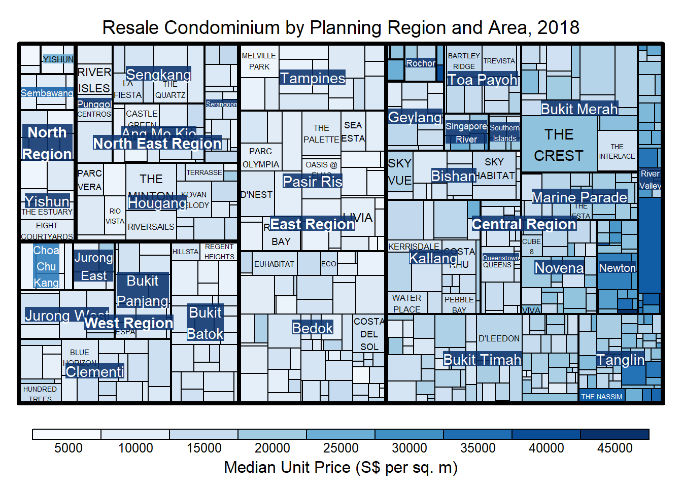
treemap(realis2018_selected,
        index = c("Planning Region", "Planning Area", "Project Name"),
        vSize = "Total Unit Sold",
        vColor = "Median Unit Price ($ psm)",
        type = "manual",
        palette = "Blues",
        algorithm = "pivotSize",
        sortID = "Median Transacted Price",
        title = "Resale Condominium by Planning Region and Area, 2018",
        title.legend = "Median Unit Price (S$ per sq. m)")
NoteThings to learn from the code chunk above
sortID = "Median Transacted Price" orders rectangles within each parent by transacted price, so the most expensive projects appear first.
16.5 Designing Treemap using treemapify Package
treemapify provides treemap geoms inside the ggplot2 grammar, which is convenient when the rest of the workflow uses ggplot2.
16.5.1 Designing a Basic Treemap
The minimal geom_treemap() call.
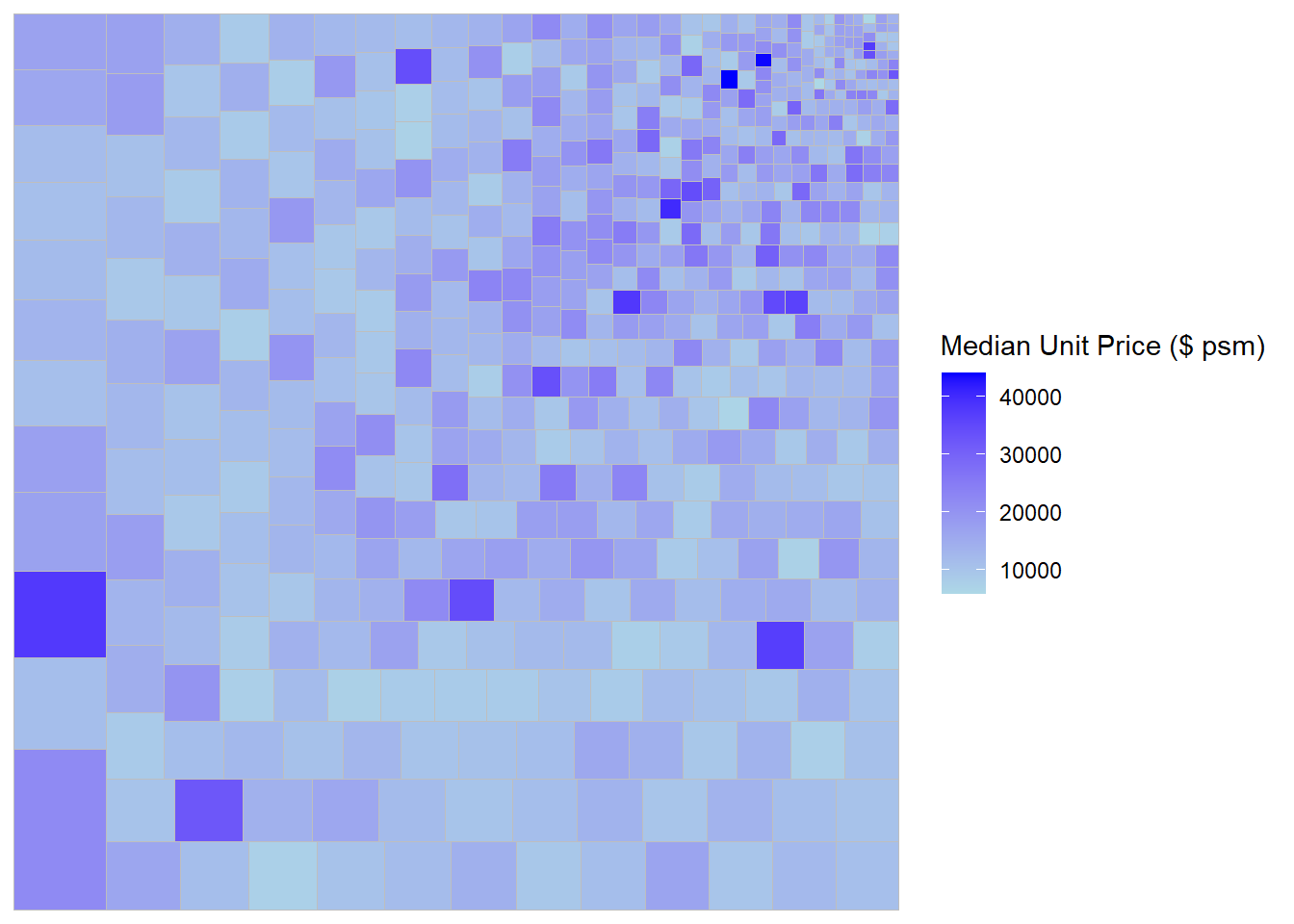
ggplot(data = realis2018_selected,
       aes(area = `Total Unit Sold`,
           fill = `Median Unit Price ($ psm)`),
       layout = "scol",
       start = "bottomleft") +
  geom_treemap() +
  scale_fill_gradient(low = "light blue", high = "blue")
NoteThings to learn from the code chunk above
The area aesthetic replaces vSize and the fill aesthetic replaces vColor. scale_fill_gradient(low = "light blue", high = "blue") creates a sequential palette. layout = "scol" and start = "bottomleft" control the rectangle placement order.
16.5.2 Defining Hierarchy
The hierarchy is added with subgroup and subgroup2. Group by Planning Region.
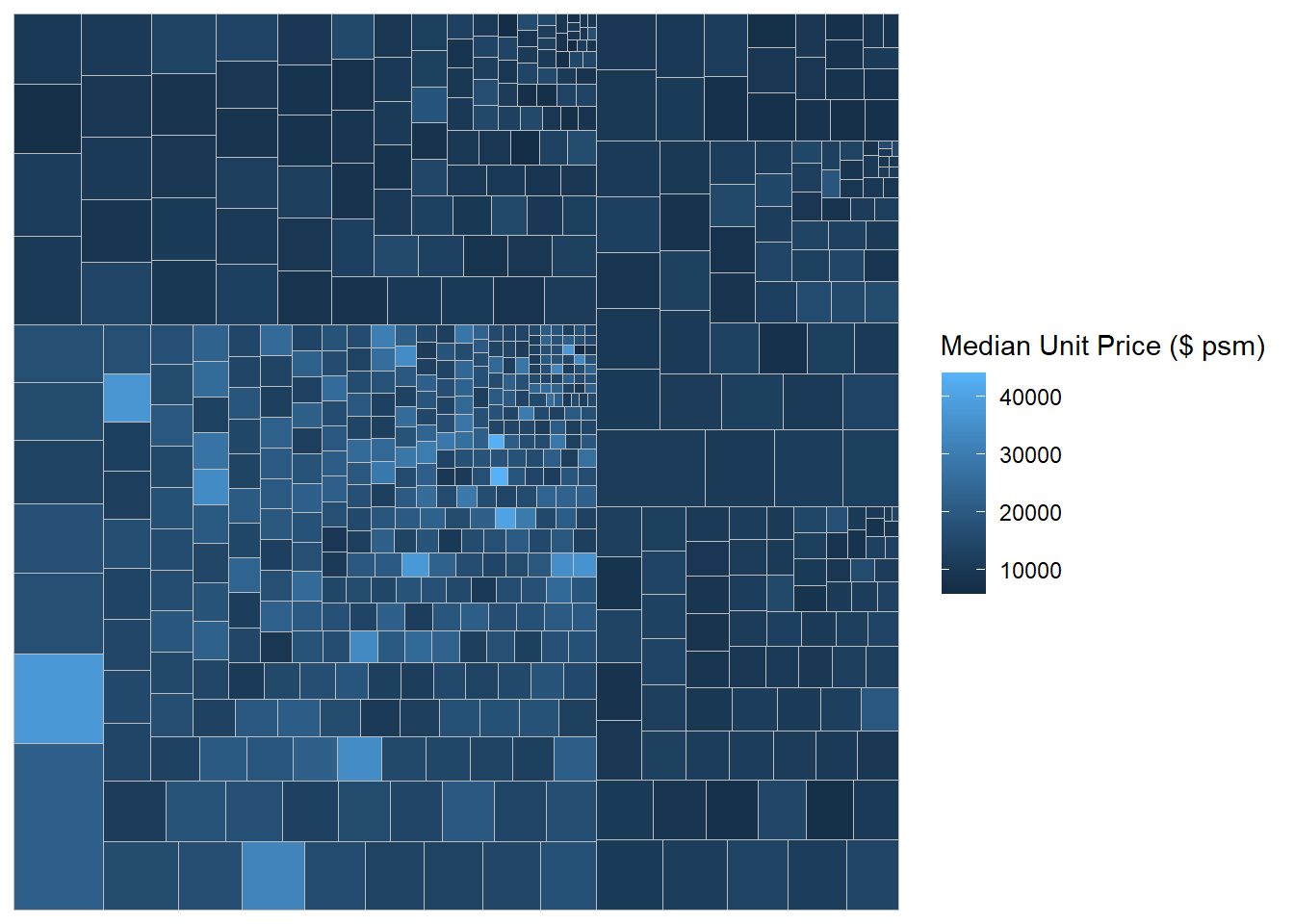
ggplot(data = realis2018_selected,
       aes(area = `Total Unit Sold`,
           fill = `Median Unit Price ($ psm)`,
           subgroup = `Planning Region`),
       start = "topleft") +
  geom_treemap()
Group by Planning Region and Planning Area.
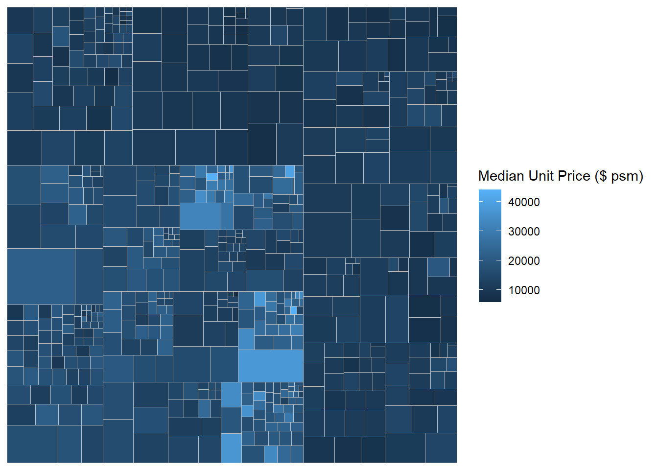
ggplot(data = realis2018_selected,
       aes(area = `Total Unit Sold`,
           fill = `Median Unit Price ($ psm)`,
           subgroup = `Planning Region`,
           subgroup2 = `Planning Area`)) +
  geom_treemap()
Adding boundary lines makes the hierarchy explicit.
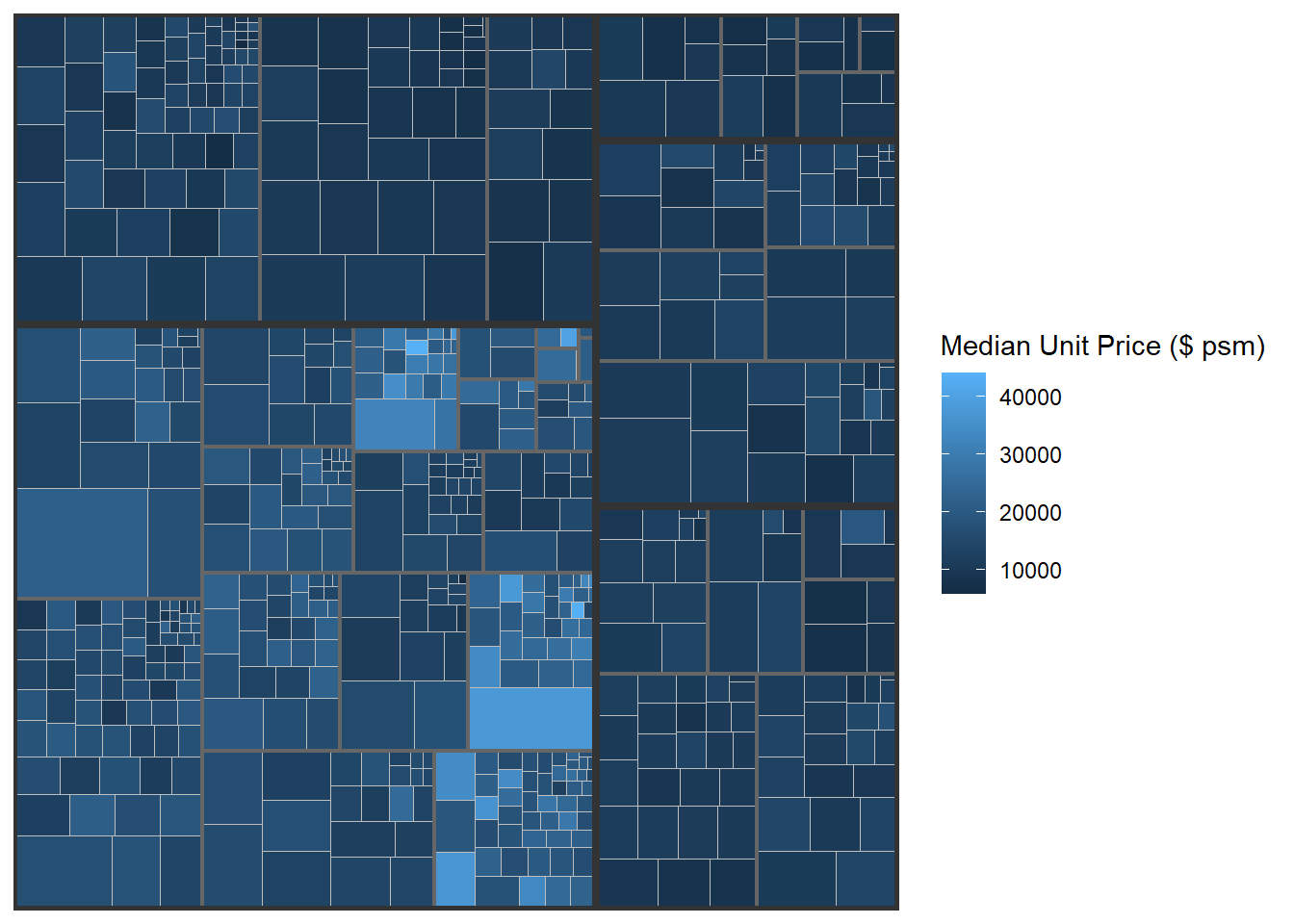
ggplot(data = realis2018_selected,
       aes(area = `Total Unit Sold`,
           fill = `Median Unit Price ($ psm)`,
           subgroup = `Planning Region`,
           subgroup2 = `Planning Area`)) +
  geom_treemap() +
  geom_treemap_subgroup2_border(colour = "gray40", size = 2) +
  geom_treemap_subgroup_border(colour = "gray20")
NoteThings to learn from the code chunk above
geom_treemap_subgroup_border() and geom_treemap_subgroup2_border() draw boundaries at the two hierarchy levels. The thicker outer border separates planning regions and the thinner inner border separates planning areas within each region.
TipReading the plot
The hierarchy is now visually accessible in three layers: region (outer borders), area (inner borders), and project (individual rectangles). A reader can scan from large to small to identify which region accounts for most resale volume, which area within that region dominates, and which project within that area is the largest.
16.6 Designing Interactive Treemap using d3treeR
d3treeR adds drill-down interactivity, allowing the reader to click into a region and see only its sub-areas. This is useful when deep hierarchies become unreadable at the leaf level.
16.6.1 Installing d3treeR Package
d3treeR is hosted on GitHub rather than CRAN, so installation requires devtools.
install.packages("devtools")
library(devtools)
install_github("timelyportfolio/d3treeR")
library(d3treeR)
16.6.2 Designing An Interactive Treemap
The interactive treemap is built in two steps: first, build a static treemap object; second, pass it to d3tree().
tm <- treemap(realis2018_summarised,
              index = c("Planning Region", "Planning Area"),
              vSize = "Total Unit Sold",
              vColor = "Median Unit Price ($ psm)",
              type = "value",
              title = "Private Residential Property Sold, 2018",
              title.legend = "Median Unit Price (S$ per sq. m)")

d3tree(tm, rootname = "Singapore")
NoteThings to learn from the code chunk above
d3tree() consumes a treemap object, so building the static version first means the same code supports both export formats. rootname = "Singapore" labels the top-level node, which is visible when the user has drilled all the way up.
🕹️ LEVEL COMPLETE 🕹️
★ ★ ★ ★ ★
CHAPTER 16 CLEARED!
+1000 XP · ACHIEVEMENT UNLOCKED: Treemap Tactician 🗺️
Press any key to continue…