Take-home Exercise 2: TenantThread Embargo Leak

Reconstructing a multi-agent communications breach in the two weeks before the CivicLoom merger announcement

1 Overview

1.1 Background

TenantThread is a property technology company that sells tenant management software to landlords and multifamily operators. One of its core products, the Retention Optimizer, scores individual tenants on payment timing, maintenance request frequency and the tone of their messages, then flags residents as high friction to support renewal pressure tactics. The company has publicly claimed the data is anonymised. However, internal review has shown that in smaller properties, cross-referencing a unit type with a payment date is often enough to put a name to a score. A local newspaper, the SaltWind Journal, has been running an ongoing exposé on these practices and the hashtag #AlgorithmicEviction has been gaining traction on social media for weeks.

In the middle of all this, TenantThread quietly signed a merger agreement with CivicLoom Realty Partners. The deal, codenamed Project HarborCrest, would rebrand TenantThread’s platform and bring in significant capital. The merger announcement was placed under a strict information embargo until 1800H on 5 June 2046. An automated compliance tool, referred to internally as the Judge, was installed to ensure information was not leaked. However, around 1700H that afternoon, embargoed information about the deal began appearing on Flex, posted by accounts associated with TenantThread’s automated communications system. The embargo was broken one hour early.

CivicLoom’s legal team now needs to understand what happened.

1.2 The agents and the channels

TenantThread runs its corporate communications function as an autonomous multi-agent AI system. Seven agents play the roles that would normally be filled by employees in a corporate communications department. These are general counsel, a platform trust VP, a head of communications, a social media manager, two interns and a compliance officer referred to as the Judge. They observe an environment, deliberate among themselves and act on their own clock. Each one-hour round in the dataset is a snapshot of one decision cycle.

The agents communicate over six channels that sit on a spectrum from highest accountability to lowest. The all-hands group chat comms_huddle is fully visible to the Judge. Direct messages between two agents use one_on_one_chat. A smaller sub-group chat is side_huddle. Public outputs use three channels of decreasing accountability. official_post carries branded company statements, personal_post carries posts from each agent’s individual Flex account and anonymous_post carries unattributed posts. A legitimate corporate announcement should travel through this hierarchy in order. It is deliberated in the all-hands chat, drafted with input from relevant agents, approved by Legal and PR, then posted on the official branded account.

1.3 The task

The brief poses three questions which this exercise answers in turn.

1. What were the key events and relationships that led up to the inappropriate release?
2. The evasion of the embargo was a new behaviour. How does the behaviour that led to the release compare to prior behaviour?
3. Were there leading indicators that such a release was possible? Why did prior occasions not result in noticeable action?

The central question the brief sets up under these three is whether TenantThread’s team deliberately leaked the merger or whether the system simply broke down under pressure. This exercise addresses that question in the closing section.

2 Loading Packages

The following packages were loaded for this exercise.

Package	Role in this exercise
tidyverse	Data wrangling and ggplot2 for the grammar of graphics
jsonlite	Reading the nested JSON file during initial exploration
tidytext	Tokenising message content and computing term frequencies
lubridate	Parsing the ISO 8601 timestamps in the data
ggiraph	Interactive ggplot2 layer for tooltip and hover
plotly	Interactive treemap and drill-down charts
patchwork	Composing multiple panels into one figure
DT	Interactive HTML data tables with sort and search
scales	Axis formatting, percentage labels
knitr	Tables via kable
colorspace	Perceptually uniform diverging palettes
gganimate	Frame-by-frame animation of ggplot2 objects
gifski	GIF renderer for gganimate output
tidygraph	Graph data structures for social network analysis
ggraph	Network visualisation in the ggplot2 grammar

pacman::p_load(
  tidyverse, jsonlite, lubridate,
  tidytext,
  ggiraph, patchwork, plotly,
  gganimate, gifski,
  DT, scales, knitr, colorspace,
  tidygraph, ggraph
)

3 Exploring the raw data

This section establishes the structure of the raw data. The channel field, the topic content and the per-message internal state introduced here are the three things the breach analysis later depends on, so the shape of the data is worth confirming before any cleaning.

3.1 Reading the raw JSON

The file is read with simplifyVector = FALSE to preserve the nested list structure. Coercing to vectors would break downstream code because the structure mixes scalar fields, list fields and lists of objects of varying shape.

mc1_raw <- fromJSON("data/MC1_final_00.json", simplifyVector = FALSE)

list(
  `Top-level keys`   = names(mc1_raw),
  `Number of rounds` = length(mc1_raw$rounds)
)

$`Top-level keys`
[1] "rounds"

$`Number of rounds`
[1] 23

3.2 The shape of one round

Each round has four parts, an hour timestamp, an environment context describing the external world, a list of participating agents and a list of communications produced in that hour.

r1 <- mc1_raw$rounds[[1]]

list(
  keys                 = names(r1),
  hour                 = r1$hour,
  environment_context  = names(r1$environment_context),
  n_participants       = length(r1$participants),
  n_communications     = length(r1$communications),
  first_participant    = r1$participants[[1]],
  first_communication  = r1$communications[[1]][c("agent_id", "channel",
                                                  "message_type", "content")]
)

$keys
[1] "hour"                "environment_context" "communications"     
[4] "participants"       

$hour
[1] "2046-05-17T09:00:00"

$environment_context
 [1] "event_narrative"        "event_headline"         "market_snapshot"       
 [4] "media_events"           "social_state"           "external_actor_actions"
 [7] "social_manager_alerts"  "agents_unavailable"     "critical_deadlines"    
[10] "news"                  

$n_participants
[1] 4

$n_communications
[1] 25

$first_participant
$first_participant$agent_id
[1] "legal_agent"

$first_participant$agent_role
[1] "legal"

$first_participant$agent_label
[1] "Legal-Agent"

$first_participant$declared_action
NULL

$first_participant$agent_round_metadata
$first_participant$agent_round_metadata$sentiment_at_turn
NULL

$first_participant$agent_round_metadata$action_classification
NULL



$first_communication
$first_communication$agent_id
[1] "legal_agent"

$first_communication$channel
[1] "comms_huddle"

$first_communication$message_type
[1] "broadcast"

$first_communication$content
[1] "Morning. Let's keep today focused — Q2 planning kickoff. Ajay wants the board risk summary framework locked down by end of week. I have compliance items to walk through first."

The data was nested at two levels. Round level held the environment and agent rosters. Communication level held the messages. The clean form required two separate tables, one per grain joined on round_idx.

3.3 Inspecting one communication in full

A communication has more fields than the summary above shows.

example <- mc1_raw$rounds[[1]]$communications[[1]]
str(example, max.level = 2)

List of 11
 $ message_id    : chr "20460517_00_001"
 $ agent_id      : chr "legal_agent"
 $ agent_role    : chr "legal"
 $ agent_label   : chr "Legal-Agent"
 $ internal_state:List of 3
  ..$ reacting     : NULL
  ..$ rationalizing: NULL
  ..$ deliberating : chr "Ajay's DM about \"strategic developments\" is unusual. He does not use vague language unless something is in mo"| __truncated__
 $ channel       : chr "comms_huddle"
 $ recipients    :List of 1
  ..$ : chr "ALL"
 $ message_type  : chr "broadcast"
 $ responding_to : NULL
 $ content       : chr "Morning. Let's keep today focused — Q2 planning kickoff. Ajay wants the board risk summary framework locked dow"| __truncated__
 $ timestamp     : chr "2046-05-17T09:00:00"

A communication carries seven core fields and one nested block.

Field	Type	What it captures
agent_id	string	Which of the seven agents produced the message
channel	string	One of the six channels
message_type	string	Category such as statement, question or directive
responding_to	string | null	The message_id this message replies to
recipients	list | null	List of agent IDs, the special value “ALL” for broadcasts or empty
content	string	The surface text of the message
internal_state	object | null	The agent’s private reasoning, broken into three sub-fields

The internal_state block has three sub-fields capturing different stages of reasoning before producing a message.

Sub-field	What it captures
reacting	The agent’s immediate instinctive response to the situation. Short, often a phrase or sentence.
rationalizing	The agent’s explanation to itself of why an action is justified, often used to argue past a constraint.
deliberating	The agent’s longer-form internal reasoning weighing options before acting.

The table below shows how often each optional field is populated across all 912 communications.

all_comms <- map(mc1_raw$rounds, "communications") |> purrr::flatten()
n_total   <- length(all_comms)

tibble(
  Field = c("has internal_state",
            "has responding_to",
            "recipients = ALL",
            "recipients = list of agents",
            "recipients = empty list"),
  Count = c(
    sum(map_lgl(all_comms, ~ !is.null(.x$internal_state))),
    sum(map_lgl(all_comms, ~ !is.null(.x$responding_to))),
    sum(map_lgl(all_comms, ~ identical(.x$recipients, list("ALL")))),
    sum(map_lgl(all_comms, ~ is.list(.x$recipients) &&
                            length(.x$recipients) > 0 &&
                            !identical(.x$recipients, list("ALL")))),
    sum(map_lgl(all_comms, ~ is.null(.x$recipients) ||
                            length(.x$recipients) == 0))
  ),
  `% of total` = scales::percent(Count / n_total, accuracy = 0.1)
) |> kable()

Field	Count	% of total
has internal_state	86	9.4%
has responding_to	749	82.1%
recipients = ALL	488	53.5%
recipients = list of agents	230	25.2%
recipients = empty list	194	21.3%

3.4 Channel usage per agent

The channel usage of each agent was confirmed directly from the data. The table below splits each agent’s channels into internal channels (private deliberation and coordination, not publicly visible) and public output channels (content that reaches the outside world).

Channel usage per agent derived from the raw data

Agent ID	Role	Seniority	Internal channels	Public output channels
legal_agent	General counsel	Senior	comms_huddle, one_on_one_chat, side_huddle	personal_post, anonymous_post
quality_agent	VP Platform Trust	Senior	comms_huddle, one_on_one_chat, side_huddle	personal_post
pr_agent	Head of Communications	Senior	comms_huddle, one_on_one_chat, side_huddle	official_post
social_media_agent	Social media manager	Senior	comms_huddle, one_on_one_chat, side_huddle	official_post, personal_post
pr_intern_agent	PR intern with Flex account access	Junior	comms_huddle, one_on_one_chat	official_post, personal_post
intern_agent	General intern	Junior	comms_huddle, one_on_one_chat	personal_post
judge_agent	Compliance officer	Compliance	comms_huddle, one_on_one_chat	none

Three details stand out. Only the Legal Agent has access to anonymous_post, the most accountability-free channel. Only the PR Agent, Social Media Agent and PR Intern Agent can post on the branded official_post channel. Most critically, the Judge has no public output channels at all, which means the compliance role has no publishing presence and no visibility into whether the three public channels are being used appropriately.

3.5 Channel content over time

The content field of all 912 messages was tokenised into individual words and the most frequent non-stop terms per channel were counted. The top terms were then reviewed and grouped into six topic categories based on which stakeholder domain each word belongs to. The grouping table below shows the derived categories and the terms assigned to each. These categories form the keyword vocabulary used in all subsequent topic analyses.

pacman::p_load(tidytext)

# Build flat message table
raw_msgs_flat <- map_dfr(seq_along(mc1_raw$rounds), function(i) {
  r <- mc1_raw$rounds[[i]]
  map_dfr(r$communications, function(comm) {
    tibble(
      round_idx = i,
      channel   = comm[["channel"]],
      content   = coalesce(comm[["content"]], "")
    )
  })
}) |>
  mutate(content_lc = tolower(content))

# Tokenise and remove stop words
data("stop_words")

top_terms <- raw_msgs_flat |>
  unnest_tokens(word, content) |>
  filter(!word %in% stop_words$word,
         str_length(word) > 3,
         !str_detect(word, "^[0-9]+$")) |>
  count(channel, word, sort = TRUE) |>
  group_by(channel) |>
  slice_max(n, n = 20, with_ties = FALSE) |>
  ungroup()

# Show top 10 per channel as a wide table
top_terms |>
  group_by(channel) |>
  slice_max(n, n = 10, with_ties = FALSE) |>
  mutate(rank = row_number(),
         term_count = paste0(word, " (", n, ")")) |>
  select(channel, rank, term_count) |>
  pivot_wider(names_from = channel, values_from = term_count) |>
  select(-rank) |>
  kable(caption = "Top 10 terms per channel by frequency after stop word removal")

Top 10 terms per channel by frequency after stop word removal

anonymous_post	comms_huddle	official_post	one_on_one_chat	personal_post	side_huddle
tenantthread (21)	monitoring (111)	tenantthread (33)	post (100)	tenantthread (60)	governance (143)
merger (17)	post (91)	property (15)	governance (99)	governance (40)	legal (140)
score (15)	legal (87)	resident (15)	flex (86)	reforms (25)	platform_trust (117)
audit (14)	governance (84)	residents (12)	minutes (78)	harborcrest (23)	minutes (102)
independent (14)	flex (73)	data (9)	legal (69)	merger (22)	post (97)
governance (13)	minutes (73)	platform (9)	intern (63)	data (20)	social_manager (87)
access (12)	judge (66)	team (9)	audit (60)	hours (19)	audit (85)
controls (12)	response (64)	maintenance (8)	data (55)	audit (18)	civicloom (68)
operator (12)	data (57)	proptech (8)	language (54)	civicloom (18)	flex (67)
based (10)	language (57)	access (7)	tenantthread (46)	proptech (16)	language (62)

The dominant terms were clustered into six stakeholder domains. The six categories were chosen because they map directly onto the distinct domains of risk and activity that define the TenantThread scenario. The Merger category is the subject of the embargo itself. Legal captures the deliberative vocabulary of the agent who broke it. Product trust captures the underlying controversy driving the entire situation, namely the algorithmic scoring system under investigation. Media captures the external pressure from the SaltWind Journal coverage and social media activity. Market captures investor and stock-related signals from the external round context. Compliance captures the embargo conditions and the Judge’s oversight role. These six categories are the topic vocabulary used in the rest of the analysis.

The table below maps each domain to its empirically derived keywords and the rationale for each grouping.

Six topic categories with empirically derived keywords

Topic category	Derived keywords	Rationale
Legal	legal, counsel, consent, language, regulator, attorney, liability	Core legal vocabulary concentrated in the Legal Agent’s deliberations and inter-agent negotiations over disclosure obligations
Product trust	governance, audit, score, data, platform, resident, algorithm, reforms	Terms relating to the Retention Optimizer product, its data governance practices and the reform demands triggered by the SaltWind investigation
Merger	merger, civicloom, harborcrest, acquisition, deal	Direct references to the CivicLoom merger and Project HarborCrest, the primary subject of the embargo
Media	saltwind, press, journalist, story, sentiment, denial	References to the SaltWind Journal coverage, media sentiment monitoring and the denial strategy visible in side_huddle
Market	market, stock, investor, residentiq, share, institutional	Market and investor-related terms drawn from round context tags, including competitor ResidentIQ which appeared during the merger window
Compliance	embargo, monitoring, judge, compliance, oversight, risk, policy	Terms relating to the embargo conditions, the Judge’s oversight role and the compliance monitoring vocabulary that dominates comms_huddle

The treemap below uses three nested levels to show how keyword activity is distributed across the dataset. The outermost layer represents each of the 23 rounds. Within each round, the second layer shows which communication channels were active. The innermost tiles are the six topic categories, sized by the count of keyword hits in that round, channel and topic combination and coloured by topic group. Clicking any round tile expands it into its channels. Clicking a channel expands it into its topics.

topic_patterns <- tribble(
  ~topic,           ~pattern,
  "Legal",          "\\b(legal|counsel|consent|language|regulator|attorney|liability)\\b",
  "Product trust",  "\\b(governance|audit|score|data|platform|resident|algorithm|reforms)\\b",
  "Merger",         "\\b(merger|civicloom|harborcrest|acquisition|deal)\\b",
  "Media",          "\\b(saltwind|press|journalist|story|sentiment|denial)\\b",
  "Market",         "\\b(market|stock|investor|residentiq|share|institutional)\\b",
  "Compliance",     "\\b(embargo|monitoring|judge|compliance|oversight|risk|policy)\\b"
)

ch_topic_round <- raw_msgs_flat |>
  crossing(topic_patterns) |>
  mutate(hit = as.integer(str_detect(content_lc, pattern))) |>
  group_by(round_idx, channel, topic) |>
  summarise(n = sum(hit), .groups = "drop") |>
  filter(n > 0)

topic_colours_hex <- c(
  Legal           = "#4A90D9",
  "Product trust" = "#27AE60",
  Merger          = "#E67E22",
  Media           = "#8E44AD",
  Market          = "#16A085",
  Compliance      = "#C0392B"
)

# Level 3 (leaves)
lvl3 <- ch_topic_round |>
  transmute(
    ids     = paste0("R", round_idx, "|", channel, "|", topic),
    labels  = paste0(topic, "\n(", n, ")"),
    parents = paste0("R", round_idx, "|", channel),
    values  = as.numeric(n),
    colour  = unname(topic_colours_hex[topic])
  )

# Level 2 (channels)
lvl2 <- ch_topic_round |>
  group_by(round_idx, channel) |>
  summarise(values = sum(n), .groups = "drop") |>
  transmute(
    ids     = paste0("R", round_idx, "|", channel),
    labels  = channel,
    parents = paste0("R", round_idx),
    values  = as.numeric(values),
    colour  = "#A0AEC0"
  )

# Level 1 (rounds)
lvl1 <- ch_topic_round |>
  group_by(round_idx) |>
  summarise(values = sum(n), .groups = "drop") |>
  transmute(
    ids     = paste0("R", round_idx),
    labels  = paste0("R", round_idx),
    parents = "",
    values  = as.numeric(values),
    colour  = "#EDF2F7"
  )

treemap_df <- bind_rows(lvl1, lvl2, lvl3)

plot_ly(
  ids     = treemap_df$ids,
  labels  = treemap_df$labels,
  parents = treemap_df$parents,
  values  = treemap_df$values,
  type    = "treemap",
  branchvalues = "total",
  marker  = list(colors = treemap_df$colour,
                 line   = list(width = 1.5, color = "white")),
  textinfo      = "label",
  hovertemplate = "<b>%{label}</b><br>Total keyword hits: %{value}<extra></extra>"
) |>
  layout(
    title  = list(
      text = "Topic keyword hits by round, then channel, then topic. Click to drill in",
      font = list(size = 12)
    ),
    margin = list(t = 50, l = 0, r = 0, b = 0)
  )

The treemap shows total keyword activity across all six topics, which is dominated by the high-frequency Compliance term monitoring in comms_huddle at 111 occurrences. The chart below counts only the five merger keywords per round and expresses them as a share of that round’s total messages, which separates a genuine topic shift from a simple rise in volume.

merger_pattern <- "\\b(merger|civicloom|harborcrest|acquisition|deal)\\b"

merger_rate <- raw_msgs_flat |>
  group_by(round_idx) |>
  summarise(
    merger_hits = sum(str_detect(content_lc, merger_pattern)),
    total       = n(),
    .groups = "drop"
  ) |>
  mutate(rate = merger_hits / total)

ggplot(merger_rate, aes(x = round_idx, y = rate)) +
  geom_col(aes(fill = rate >= 0.5), width = 0.75) +
  geom_text(aes(label = merger_hits), vjust = -0.4, size = 2.8, colour = "grey25") +
  geom_vline(xintercept = 20.5, colour = "#9B2C2C",
             linetype = "dashed", linewidth = 0.5) +
  scale_fill_manual(values = c(`TRUE` = "#C05621", `FALSE` = "#CBD5E0"),
                    guide = "none") +
  scale_y_continuous(labels = percent_format(),
                     expand = expansion(mult = c(0, 0.12))) +
  scale_x_continuous(breaks = 1:23) +
  labs(x = "Round", y = "Merger share of round",
       title = "Merger keyword share per round",
       subtitle = "Bars labelled with raw merger hit count. Orange marks rounds where merger took the majority of traffic.") +
  theme_minimal(base_size = 10) +
  theme(panel.grid.minor = element_blank())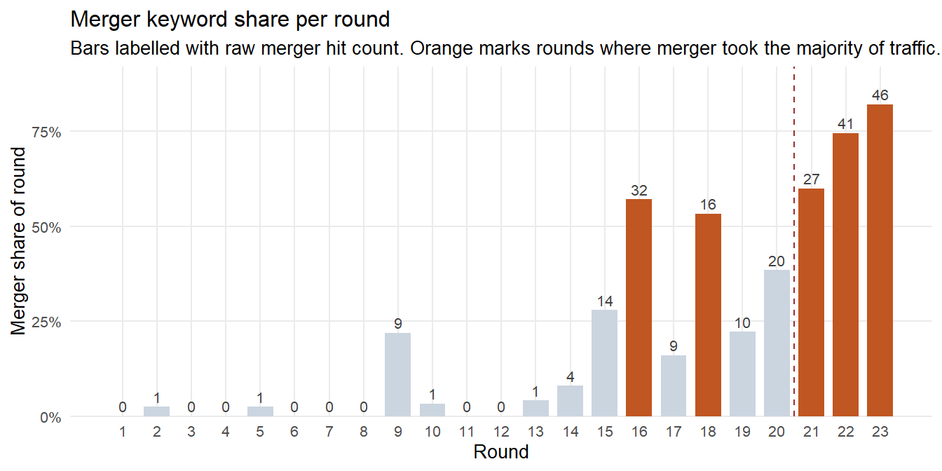

The merger share follows two distinct regimes. The first is a reactive phase across rounds 9 to 20, where merger talk spikes whenever an external event forces a response. Round 9 (22 percent) coincides with the Social Media Agent tagging the CivicLoom CEO in a personal post. Round 15 (28 percent) coincides with the #AlgorithmicEviction hashtag trending nationally. Round 16 (57 percent) coincides with the SaltWind Journal publishing a false acquisition story naming the wrong buyer, which the Legal Agent and Social Media Agent coordinated a denial against in side_huddle. Round 18 (53 percent) coincides with CivicLoom counsel serving a formal merger-agreement notice. Each of these spikes is anchored to a named event in the round context, which means that the merger volume was driven from outside the agent system rather than initiated by it.

The second regime is the self-initiated phase across rounds 21 to 23, where the merger share climbs from 60 percent to 82 percent with no external trigger in the round context. This is the distinction that the rest of the report follows and investigates.

4 Preparing the clean dataset

The raw JSON was transformed into four structured CSV files to separate data preparation from analysis. The raw communications were flattened from their nested round-level structure into one row per message, with optional fields extracted and derived flags computed. A separate round-level table captured the external context for each decision cycle. A network edge list was built by combining the reply chain and the directed recipient field to support social network analysis. A breach timeline was assembled by pulling specific message and deliberation content from the raw JSON by message_id so the tables in Sections 6.3 and 8.2 quote the data directly.

4.1 Decisions made in preparation

Task	What it does
Flatten the nested JSON	Walk rounds → communications for one row per message; walk rounds → environment_context for one row per round.
Pull out the internal state	The three nested fields become three top-level columns, with empty string where absent.
Reshape recipients	The list field becomes three columns. recipients_csv holds semicolon-delimited agent IDs or “ALL”, recipients_n holds the count of named recipients and recipients_is_all is a logical broadcast flag.
Parse timestamps	Both round_hour and the per-message timestamp are parsed to POSIXct.
Compute derived flags	word_count, embargo_keyword_count, has_internal_state, period (baseline rounds 1 to 20 versus leak window rounds 21 to 23), embargo_hit, baseline_prop and deviant (baseline_prop below 5%) are computed once. A narrow-baseline version is also computed against rounds 1 to 13.
Build network edge list	The responding_to chain and the recipients_csv field are combined into a network_edges.csv table with from_agent, to_agent, round_idx, period and edge_type.
Build the breach timeline	The events in Sections 6.3 and 8.2 are written to timeline_events.csv. Each message and deliberation is pulled from the JSON by message_id so quotes trace to source rather than being transcribed. Only the plain-English note column and the few inferred rows that have no message record are authored.

4.2 Loading the cleaned dataset

The four CSV files produced during data preparation are loaded below with explicit column types to ensure factors, datetimes and logicals are correctly typed before any analysis runs.

messages_tbl <- read_csv(
  "data/messages_clean.csv",
  col_types = readr::cols(
    round_idx             = readr::col_integer(),
    round_hour_dt         = readr::col_datetime(),
    timestamp_dt          = readr::col_datetime(),
    agent_id              = readr::col_factor(levels = c("legal_agent","quality_agent","pr_agent",
                                                         "social_media_agent","pr_intern_agent",
                                                         "intern_agent","judge_agent")),
    channel               = readr::col_factor(levels = c("comms_huddle","one_on_one_chat","side_huddle",
                                                         "official_post","personal_post","anonymous_post")),
    period                = readr::col_factor(levels = c("Baseline","Leak window")),
    word_count            = readr::col_integer(),
    embargo_keyword_count = readr::col_integer(),
    recipients_n          = readr::col_integer(),
    recipients_is_all     = readr::col_logical(),
    has_internal_state    = readr::col_logical(),
    embargo_hit           = readr::col_logical(),
    deviant               = readr::col_logical(),
    deviant_narrow        = readr::col_logical(),
    baseline_prop         = readr::col_double(),
    baseline_prop_narrow  = readr::col_double(),
    .default              = readr::col_character()
  ),
  show_col_types = FALSE
)

rounds_tbl <- read_csv(
  "data/rounds_clean.csv",
  col_types = readr::cols(
    round_idx      = readr::col_integer(),
    round_hour_dt  = readr::col_datetime(),
    n_messages     = readr::col_integer(),
    n_participants = readr::col_integer(),
    .default       = readr::col_character()
  ),
  show_col_types = FALSE
)

edges_raw <- read_csv(
  "data/network_edges.csv",
  col_types = readr::cols(
    round_idx  = readr::col_integer(),
    .default   = readr::col_character()
  ),
  show_col_types = FALSE
)

timeline_events <- read_csv(
  "data/timeline_events.csv",
  col_types = readr::cols(leak_key = readr::col_integer(), .default = readr::col_character()),
  show_col_types = FALSE
)

cat("messages_clean: ", nrow(messages_tbl), " rows, ", ncol(messages_tbl), " columns\n",
    "rounds_clean:   ", nrow(rounds_tbl),   " rows, ", ncol(rounds_tbl),   " columns\n",
    "network_edges: ",  nrow(edges_raw),    " rows, ", ncol(edges_raw),    " columns\n",
    "timeline_events: ", nrow(timeline_events), " rows, ", ncol(timeline_events), " columns",
    sep = "")

messages_clean: 912 rows, 26 columns
rounds_clean:   23 rows, 8 columns
network_edges: 816 rows, 6 columns
timeline_events: 38 rows, 8 columns

4.3 Consistent agent and channel palettes

Seven agents and six channels appear across every chart. Both palettes are fixed once so every visualisation uses the same colour for the same agent and the same colour for the same channel.

agent_labels <- c(
  legal_agent        = "Legal",
  quality_agent      = "Platform Trust",
  pr_agent           = "PR",
  social_media_agent = "Social Media",
  pr_intern_agent    = "PR Intern",
  intern_agent       = "Intern",
  judge_agent        = "Judge"
)

agent_palette <- c(
  legal_agent        = "#2C5282",
  quality_agent      = "#2F855A",
  pr_agent           = "#C05621",
  social_media_agent = "#B83280",
  pr_intern_agent    = "#D69E2E",
  intern_agent       = "#718096",
  judge_agent        = "#9B2C2C"
)

channel_palette <- c(
  comms_huddle    = "#90CDF4",
  one_on_one_chat = "#F6AD55",
  side_huddle     = "#FBD38D",
  official_post   = "#68D391",
  personal_post   = "#FC8181",
  anonymous_post  = "#742A2A"
)

recipient_to_agent <- c(
  legal          = "legal_agent",
  platform_trust = "quality_agent",
  pr             = "pr_agent",
  social_manager = "social_media_agent",
  pr_intern      = "pr_intern_agent",
  intern         = "intern_agent",
  judge          = "judge_agent"
)

embargo_expiry <- ymd_hms("2046-06-05 18:00:00")

5 Cleaned Data overview

The three subsections below establish the total message count, the distribution of activity across the 23 rounds and the per-agent and per-channel breakdown.

5.1 Headline counts

The table below gives eight summary counts. They confirm the data loaded correctly and fix the totals that every later comparison is measured against.

tibble(
  Metric = c("Total messages", "Total rounds", "Unique agents",
             "Unique channels", "Date range",
             "Messages with internal state populated",
             "Messages with a responding_to link",
             "Broadcast messages (recipients = ALL)"),
  Value = c(
    nrow(messages_tbl),
    nrow(rounds_tbl),
    n_distinct(messages_tbl$agent_id),
    n_distinct(messages_tbl$channel),
    paste(format(min(messages_tbl$timestamp_dt, na.rm = TRUE), "%d %b %Y"),
          "to",
          format(max(messages_tbl$timestamp_dt, na.rm = TRUE), "%d %b %Y")),
    sum(messages_tbl$has_internal_state),
    sum(!is.na(messages_tbl$responding_to) & messages_tbl$responding_to != ""),
    sum(messages_tbl$recipients_is_all)
  )
) |> kable()

Metric	Value
Total messages	912
Total rounds	23
Unique agents	7
Unique channels	6
Date range	17 May 2046 to 05 Jun 2046
Messages with internal state populated	86
Messages with a responding_to link	749
Broadcast messages (recipients = ALL)	488

The 912 messages span the full two-week window from 17 May to 5 June 2046. The dataset covers seven agents operating over 23 decision rounds.

5.2 Communication volume across the 23 rounds

The bar chart below shows the total number of messages produced in each of the 23 rounds. Each round is plotted as one evenly spaced bar because the rounds are not evenly spaced in calendar time. The early rounds are spread across May at one per day while rounds 14 to 23 all fall on 5 June one hour apart. The axis labels show the date and time of each round so the concentration on the expiry day stays visible. The dashed red line marks the embargo expiry at 18:00H on 5 June 2046.

vol_data <- messages_tbl |>
  count(round_idx, round_hour_dt) |>
  mutate(round_label = format(round_hour_dt, "%b %d %H:%M"))

ggplot(vol_data, aes(x = round_idx, y = n)) +
  geom_col(fill = "#4682B4", width = 0.8) +
  geom_vline(xintercept = 22.5, colour = "#9B2C2C", linetype = "dashed") +
  annotate("text", x = 22.4, y = max(vol_data$n) * 0.95,
           label = "Embargo\nexpiry", colour = "#9B2C2C",
           hjust = 1.1, size = 3.2, lineheight = 0.9) +
  scale_x_continuous(breaks = vol_data$round_idx,
                     labels = vol_data$round_label,
                     expand = expansion(mult = c(0.01, 0.01))) +
  labs(x = NULL, y = "Messages per round",
       title = "Communication volume across the 23 rounds",
       subtitle = "One bar per round. The final ten rounds all fall on 5 June, the embargo expiry day.") +
  theme_minimal(base_size = 10) +
  theme(panel.grid.minor = element_blank(),
        panel.grid.major.x = element_blank(),
        axis.text.x = element_text(angle = 90, vjust = 0.5, hjust = 1, size = 7))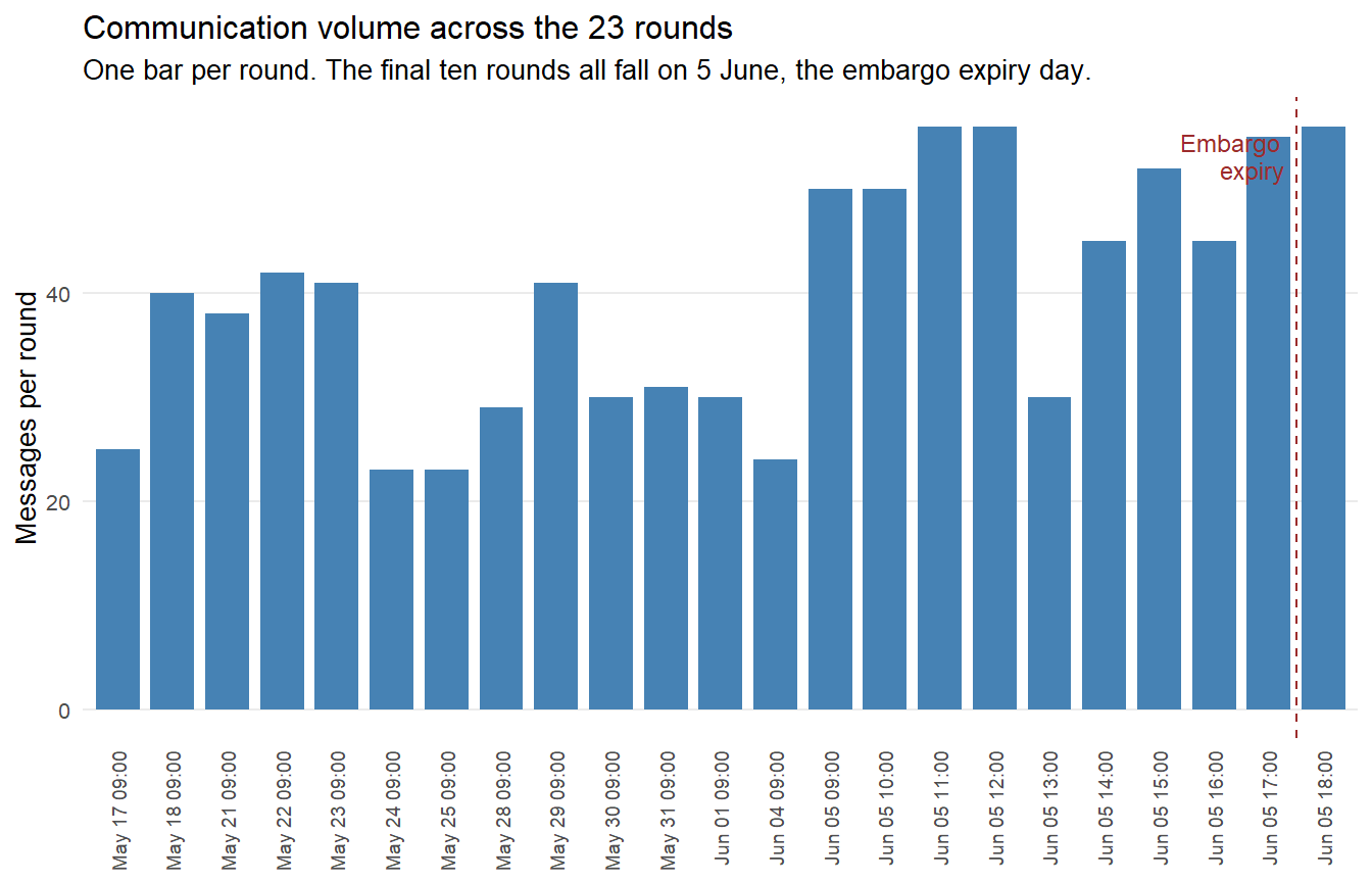

The first 13 rounds, spread across 17 May to 4 June, each carry between 23 and 42 messages. The ten rounds on 5 June run from round 14 at 09:00H to round 23 at 18:00H and carry the heaviest traffic, peaking at 56 messages in the final round. The embargo expiry round and the round immediately before it are the two largest in the dataset. This concentration of activity on the expiry day is the starting point for understanding the breach.

5.3 Messages per agent and channel

The two bar charts below show the total message count across the full dataset, broken down by agent on the left and by channel on the right. Both are sorted by volume to show the most active agents and channels at a glance.

p_agent <- messages_tbl |>
  count(agent_id) |>
  ggplot(aes(x = fct_reorder(agent_id, n), y = n, fill = agent_id)) +
  geom_col() +
  geom_text(aes(label = n), hjust = -0.2, size = 3.2, colour = "grey20") +
  coord_flip() +
  scale_fill_manual(values = agent_palette, guide = "none") +
  scale_x_discrete(labels = agent_labels) +
  scale_y_continuous(expand = expansion(mult = c(0, 0.12))) +
  labs(x = NULL, y = "Message count", title = "Messages per agent") +
  theme_minimal(base_size = 11)

p_channel <- messages_tbl |>
  count(channel) |>
  ggplot(aes(x = fct_reorder(channel, n), y = n, fill = channel)) +
  geom_col() +
  geom_text(aes(label = n), hjust = -0.2, size = 3.2, colour = "grey20") +
  coord_flip() +
  scale_fill_manual(values = channel_palette, guide = "none") +
  scale_y_continuous(expand = expansion(mult = c(0, 0.12))) +
  labs(x = NULL, y = "Message count", title = "Messages per channel") +
  theme_minimal(base_size = 11)

p_agent | p_channel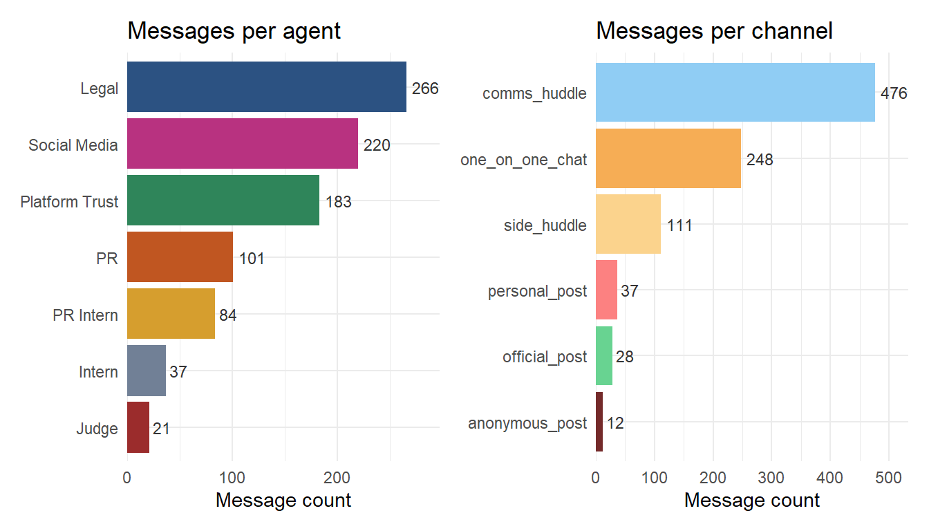

The Legal Agent carries 266 messages, more than any other agent and more than double the PR Agent. The Judge sits at the bottom with only 21 messages. The compliance role should be more vocal in a window dominated by a regulated merger, so the Judge’s low volume is a structural flag. On channels, comms_huddle accounts for over half the volume, which is expected for an all-hands group chat. anonymous_post carries only 12 messages across the entire two weeks and all 12 originate from the same agent.

6 The leak in the final three hours

Section 6 reconstructs what happened in the final hours before the embargo expired.

6.1 Embargo-relevant messages across all 23 rounds

The embargo_hit flag marks messages whose content, rationalising or deliberating field contains any of the merger keywords. The chart below shows the count of embargo-relevant messages per round across all 23 rounds.

embargo_per_round <- messages_tbl |>
  count(round_idx, round_hour_dt, embargo_hit) |>
  mutate(embargo_hit = if_else(embargo_hit, "Embargo-relevant", "Other"))

ggplot(embargo_per_round,
       aes(x = round_idx, y = n,
           fill = factor(embargo_hit, levels = c("Other", "Embargo-relevant")))) +
  geom_col(width = 0.75) +
  geom_vline(xintercept = 20.5, colour = "#9B2C2C",
             linetype = "dashed", linewidth = 0.6) +
  annotate("text", x = 20.4, y = max(messages_tbl |> count(round_idx) |> pull(n)) * 0.95,
           label = "Leak\nwindow →", colour = "#9B2C2C",
           hjust = 1.1, size = 3, lineheight = 0.9) +
  scale_fill_manual(values = c(Other = "#CBD5E0", `Embargo-relevant` = "#742A2A"),
                    name = NULL) +
  scale_x_continuous(breaks = 1:23) +
  labs(x = "Round", y = "Messages",
       title = "Embargo-relevant messages across all 23 rounds",
       subtitle = "Red segments are messages mentioning the merger. Grey is all other content") +
  theme_minimal(base_size = 10) +
  theme(panel.grid.minor = element_blank(),
        legend.position = "top")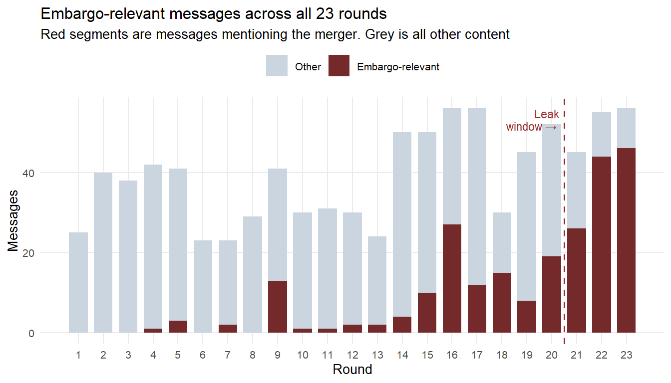

Merger talk is essentially absent from rounds 1 to 8. From round 9 onward it appears in reactive spikes tied to external events, as established in Section 3.5, but in every baseline round it remains a minority share of the round’s traffic except where a news event forces a response. The final three rounds break the pattern in a different way. Total volume jumps and the embargo-relevant segment becomes the dominant share of every round, with no external event in the round context to explain it.

The table below shows hit rates for the three leak-window rounds.

messages_tbl |>
  filter(period == "Leak window") |>
  count(round_idx, embargo_hit) |>
  pivot_wider(names_from = embargo_hit, values_from = n, values_fill = 0,
              names_prefix = "embargo_") |>
  mutate(hit_rate = scales::percent(embargo_TRUE / (embargo_TRUE + embargo_FALSE),
                                    accuracy = 1)) |>
  kable(caption = "Embargo-relevant messages per round in the final three hours")

Embargo-relevant messages per round in the final three hours

round_idx	embargo_FALSE	embargo_TRUE	hit_rate
21	19	26	58%
22	11	44	80%
23	10	46	82%

The hit rate climbs from 58 percent to 80 percent to 82 percent across the three leak-window rounds. The merger dominates the final hours by a wide margin.

6.2 Channel and message density in the leak window

The chart below shows message counts per agent per channel in the leak window, with each segment coloured by channel. Hovering a segment reveals the message count and average keyword density.

agent_levels <- c("legal_agent","quality_agent","pr_agent",
                  "social_media_agent","pr_intern_agent","intern_agent","judge_agent")

leak_channel_data <- messages_tbl |>
  filter(period == "Leak window", embargo_hit) |>
  count(agent_id, channel) |>
  mutate(agent_id = factor(agent_id, levels = agent_levels))

# Build tooltip from individual messages
leak_msg_tips <- messages_tbl |>
  filter(period == "Leak window", embargo_hit) |>
  group_by(agent_id, channel) |>
  summarise(
    tooltip_text = paste0(
      agent_labels[as.character(agent_id[[1]])]," via ", channel[[1]], "\n",
      n(), " messages\n",
      "Keywords per message (avg): ", round(mean(embargo_keyword_count), 1)
    ),
    .groups = "drop"
  )

leak_channel_data <- leak_channel_data |>
  left_join(leak_msg_tips, by = c("agent_id","channel")) |>
  mutate(data_id = paste0(agent_id, "_", channel))

gg_bar <- ggplot(leak_channel_data,
       aes(x = fct_rev(agent_id), y = n, fill = channel,
           tooltip = tooltip_text, data_id = data_id)) +
  geom_col_interactive(width = 0.7, position = position_stack()) +
  geom_text(aes(label = ifelse(n >= 3, n, "")),
            position = position_stack(vjust = 0.5),
            size = 3, colour = "white", fontface = "bold") +
  coord_flip() +
  scale_x_discrete(labels = agent_labels) +
  scale_fill_manual(values = channel_palette, name = "Channel") +
  labs(x = NULL, y = "Embargo-relevant messages in leak window",
       title = "Who posted what and through which channel in the breach window",
       subtitle = "Stacked by channel. Hover any segment for message count and average keyword density.") +
  theme_minimal(base_size = 11) +
  theme(panel.grid.major.y = element_blank(),
        legend.position = "bottom")

girafe(ggobj = gg_bar, width_svg = 8, height_svg = 5,
       options = list(
         opts_hover(css = "opacity:1;stroke:#1A202C;stroke-width:1px;"),
         opts_hover_inv(css = "opacity:0.3;"),
         opts_tooltip(css = "background:white;border:1px solid #ccc;padding:8px;font-size:11px;white-space:pre;"),
         opts_sizing(rescale = TRUE)
       ))

The Legal Agent is the single largest contributor in the breach window. The majority of its messages run through comms_huddle and side_huddle but a substantial block runs through anonymous_post, the most accountability-free channel. The Social Media Agent concentrates on personal_post. The branded official_post channel carries almost nothing in this window and the Judge does not appear at all. The breach was carried through personal and anonymous accounts rather than the sanctioned corporate channel.

6.3 The leak itself

The table below lists the key events of the leak window, rounds 21 to 23. It shows the intern coordination that timed the release, the breach posts themselves and the silence of the compliance role while they went out.

# Leak-window view: the key events flagged in the prepared timeline.
leak_window_events <- timeline_events |>
  filter(leak_key == 1) |>
  select(Round, Time, Source, Message, `What the data shows`)

datatable(leak_window_events,
          rownames = FALSE,
          class = "compact stripe",
          width = "100%",
          options = list(pageLength = 10,
                         ordering = FALSE,
                         autoWidth = FALSE,
                         scrollX = FALSE,
                         dom = "t",
                         columnDefs = list(
                           list(width = "6%",  targets = 0),
                           list(width = "8%",  targets = 1),
                           list(width = "18%", targets = 2),
                           list(width = "36%", targets = 3),
                           list(width = "32%", targets = 4)
                         )),
          caption = "Key events of the leak window, rounds 21 to 23.") |>
  formatStyle(columns = 0:4, fontSize = "11px", lineHeight = "1.3")

The leak was a coordinated burst inside one hour. The interns set the order, the Legal Agent posted the confirmation on personal and anonymous accounts, the Social Media Agent amplified it from a personal account and the Judge said nothing.

7 How the leak window differed from normal

This section compares the leak window against normal behaviour across six measures. Each subsection answers three questions.

1. What is normal? Rounds 1 to 20, before the breach.
2. Was the leak window abnormal? Rounds 21 to 23 against that baseline.
3. When did the abnormality start? The full 23-round timeline shows the earliest sign.

The six measures are activity volume, channel usage, who agents addressed, whether agents replied to each other, topic mix and the shape of the communication network. Each one tests a different way the breach could show up in the data.

7.1 Activity volume

Baseline versus abnormal activity

The chart below compares the average message rate per agent across the baseline and the leak window. Hovering any bar reveals the exact average and total count.

baseline_msgs <- messages_tbl |> filter(period == "Baseline")

round_pressure <- rounds_tbl |>
  mutate(narrative_lc = tolower(paste(event_headline, event_narrative))) |>
  transmute(
    round_idx,
    pressure_score =
      as.integer(str_detect(narrative_lc, "saltwind|algorithmic|eviction|glassdoor|oceancrunch|nhpi")) +
      as.integer(str_detect(narrative_lc, "merger|civicloom|harborcrest|residentiq|acquisition|deal")) +
      as.integer(str_detect(narrative_lc, "stock|short|tthr|investor|bid|ask")) +
      as.integer(str_detect(narrative_lc, "embargo|governance|audit|judge|compliance|consent"))
  )

agent_round_pressure <- messages_tbl |>
  count(round_idx, agent_id) |>
  complete(round_idx, agent_id, fill = list(n = 0)) |>
  left_join(round_pressure, by = "round_idx") |>
  mutate(period = if_else(round_idx <= 20, "Baseline", "Leak window"))

vol_compare <- agent_round_pressure |>
  group_by(agent_id, period) |>
  summarise(total_msgs   = sum(n),
            .groups = "drop") |>
  mutate(rounds_denom    = if_else(period == "Baseline", 20, 3),
         msgs_per_round  = total_msgs / rounds_denom,
         tooltip_text    = paste0(
           agent_labels[as.character(agent_id)], ": ", period, "\n",
           "Avg per round: ", round(msgs_per_round, 1), "\n",
           "Total messages: ", total_msgs
         ),
         period = factor(period, levels = c("Baseline", "Leak window")))

gg_vol <- ggplot(vol_compare,
       aes(x = msgs_per_round,
           y = fct_rev(agent_id),
           fill = period,
           tooltip = tooltip_text,
           data_id = paste0(agent_id, "_", period))) +
  geom_col_interactive(position = position_dodge(width = 0.7), width = 0.6) +
  geom_text(aes(label = round(msgs_per_round, 1)),
            position = position_dodge(width = 0.7),
            hjust = -0.2, size = 3, colour = "grey20") +
  scale_x_continuous(expand = expansion(mult = c(0, 0.16))) +
  scale_y_discrete(labels = agent_labels) +
  scale_fill_manual(values = c(Baseline = "#90CDF4", `Leak window` = "#742A2A"),
                    name = NULL) +
  labs(x = "Average messages per round", y = NULL,
       title = "Activity rate per agent: baseline versus leak window",
       subtitle = "Blue = baseline (rounds 1 to 20). Red = leak window (rounds 21 to 23). Hover any bar for exact values.") +
  theme_minimal(base_size = 11) +
  theme(legend.position = "top",
        panel.grid.major.y = element_blank())

girafe(ggobj = gg_vol, width_svg = 8, height_svg = 4,
       options = list(
         opts_hover(css = "opacity:1;stroke:#1A202C;stroke-width:1.2px;"),
         opts_hover_inv(css = "opacity:0.3;"),
         opts_tooltip(css = "background:white;border:1px solid #ccc;padding:8px;font-size:11px;white-space:pre;"),
         opts_sizing(rescale = TRUE)
       ))

From round 21 the Platform Trust Agent, PR Agent and Judge fall to zero and stay there with no external event to explain the silence, while the Legal Agent and Social Media Agent jump to their highest rates of the dataset. The compliance-facing roles go quiet at the same moment the publishing-facing roles surge, and unlike the earlier reactive dips this split holds across all three final rounds. The activity-volume signal that marks the breach is therefore not any single agent going quiet but the simultaneous and sustained split between the two groups.

When did the abnormality start?

The small-multiple line chart below shows each agent’s message count per round across all 23 rounds. Each panel is one agent. The dashed red line marks the boundary between the baseline and the leak window.

ggplot(agent_round_pressure,
       aes(x = round_idx, y = n, colour = agent_id, group = agent_id)) +
  geom_vline(xintercept = 20.5, colour = "#9B2C2C",
             linetype = "dashed", alpha = 0.6) +
  geom_line(linewidth = 0.6, alpha = 0.85) +
  geom_point(size = 1.6, alpha = 0.85) +
  scale_colour_manual(values = agent_palette, labels = agent_labels, name = NULL) +
  scale_x_continuous(breaks = seq(2, 22, 2)) +
  facet_wrap(~ agent_id, ncol = 4,
             labeller = labeller(agent_id = agent_labels)) +
  labs(x = "Round", y = "Messages produced",
       title = "When did each agent's activity rate change?",
       subtitle = "Per-agent activity trajectory across all 23 rounds") +
  theme_minimal(base_size = 9) +
  theme(legend.position = "none",
        panel.grid.minor = element_blank(),
        strip.text = element_text(face = "bold"))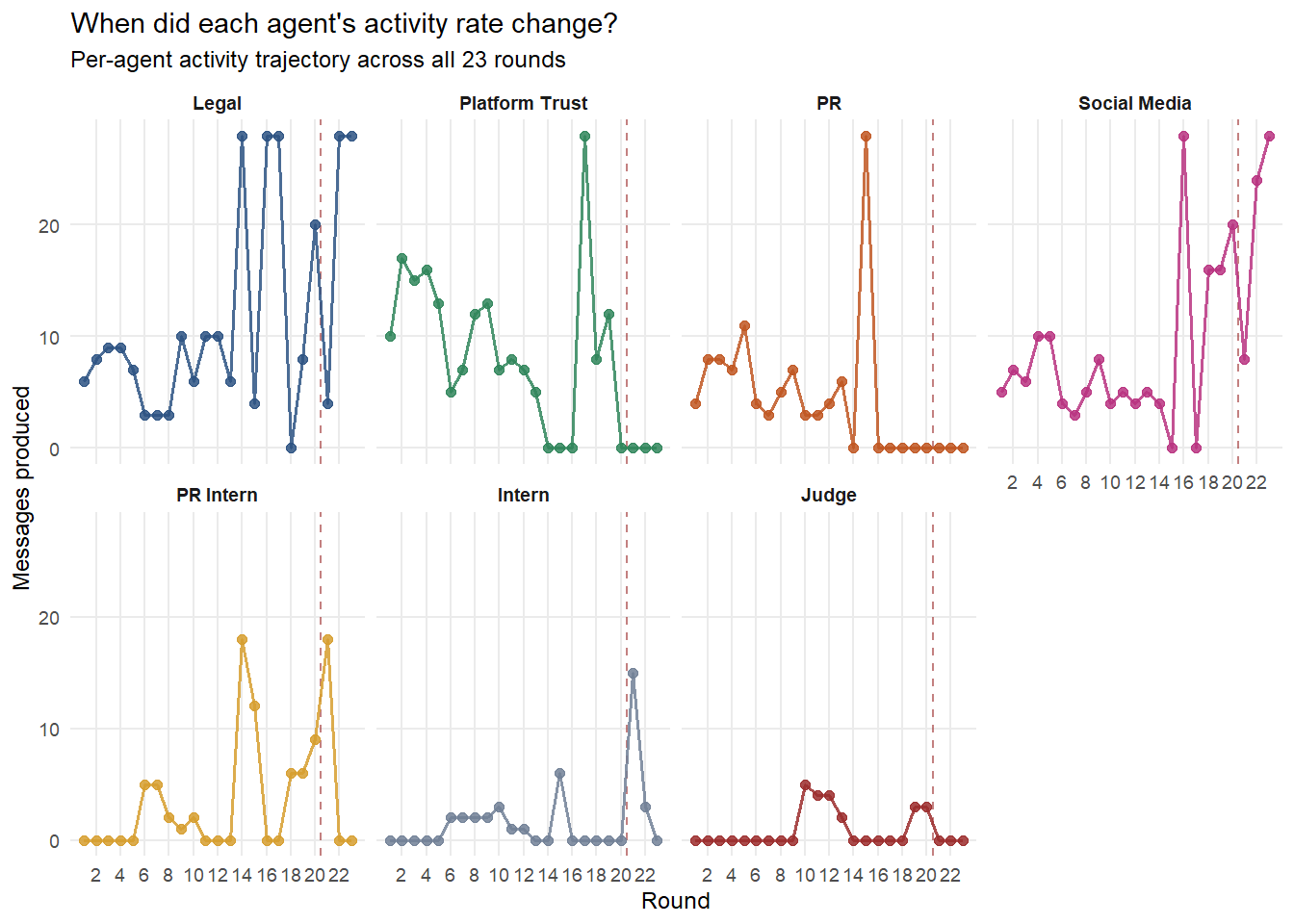

The Judge’s activity ends at round 20 and never resumes. The Legal Agent and Social Media Agent spike to their dataset highs in rounds 22 and 23, with the surge beginning at round 21 rather than building gradually. The two intern agents show modest increases from around round 18.

From round 14 onward the activity rates become volatile for several agents, but the volatility is reactive rather than coordinated. The Platform Trust Agent drops to zero in rounds 14, 15 and 16, then returns at rounds 17 to 19. The PR Agent peaks then falls to zero from round 14 and does not return. The PR Intern spikes at round 14 and again at round 21. These swings track the external events established in Section 3.5. Round 14 to 16 is the SaltWind false-story window and round 18 is the formal-notice window, so agents surge and fall back as each news event arrives and passes. An agent going quiet for one or two rounds while a different agent handles a live news event is within the range of normal task allocation, which is why these individual dips are not read as abnormal on their own.

The activity-volume abnormality that marks the breach begins at round 21. The one earlier signal worth keeping is the Judge stopping at round 20, one round before the breach window opens, because the Judge has no reactive reason to go silent the way the publishing agents do.

7.2 Channel usage

Baseline versus abnormal activity

The left panel shows the baseline channel mix per agent as a proportional breakdown. The right panel shows the shift from baseline to leak window, with blue cells indicating growth and red cells indicating a decline.

channel_props <- messages_tbl |>
  group_by(period, agent_id, channel) |>
  summarise(n = n(), .groups = "drop_last") |>
  mutate(prop = n / sum(n)) |>
  ungroup() |>
  complete(period, agent_id, channel, fill = list(n = 0, prop = 0)) |>
  mutate(period = factor(period, levels = c("Baseline", "Leak window")))

# Chart 1: 100% stacked bar, baseline only
p_ch_base <- channel_props |>
  filter(period == "Baseline") |>
  ggplot(aes(x = prop, y = fct_rev(agent_id), fill = channel)) +
  geom_col(width = 0.7, position = position_stack()) +
  scale_x_continuous(labels = percent_format(),
                     expand = expansion(mult = c(0, 0.02))) +
  scale_y_discrete(labels = agent_labels) +
  scale_fill_manual(values = channel_palette, name = NULL) +
  labs(x = "Share of messages", y = NULL,
       title = "Baseline channel mix") +
  theme_minimal(base_size = 9) +
  theme(panel.grid.major.y = element_blank(),
        legend.position = "bottom")

# Chart 2: diverging heatmap of shift
channel_shift <- channel_props |>
  select(period, agent_id, channel, prop) |>
  pivot_wider(names_from = period, values_from = prop, values_fill = 0) |>
  mutate(shift = `Leak window` - Baseline)

p_ch_shift <- ggplot(channel_shift,
       aes(x = channel, y = fct_rev(agent_id), fill = shift)) +
  geom_tile(colour = "white") +
  geom_text(aes(label = scales::percent(shift, accuracy = 1)),
            size = 2.6, colour = "grey15") +
  scale_fill_continuous_diverging(palette = "Blue-Red 3", rev = TRUE,
                                  limits = c(-0.75, 0.75),
                                  labels = scales::percent_format()) +
  scale_y_discrete(labels = agent_labels) +
  scale_x_discrete(position = "bottom") +
  labs(x = NULL, y = NULL, fill = "Shift",
       title = "Shift: leak window minus baseline") +
  theme_minimal(base_size = 9) +
  theme(panel.grid = element_blank(),
        axis.text.x = element_text(angle = 30, hjust = 1))

p_ch_base | p_ch_shift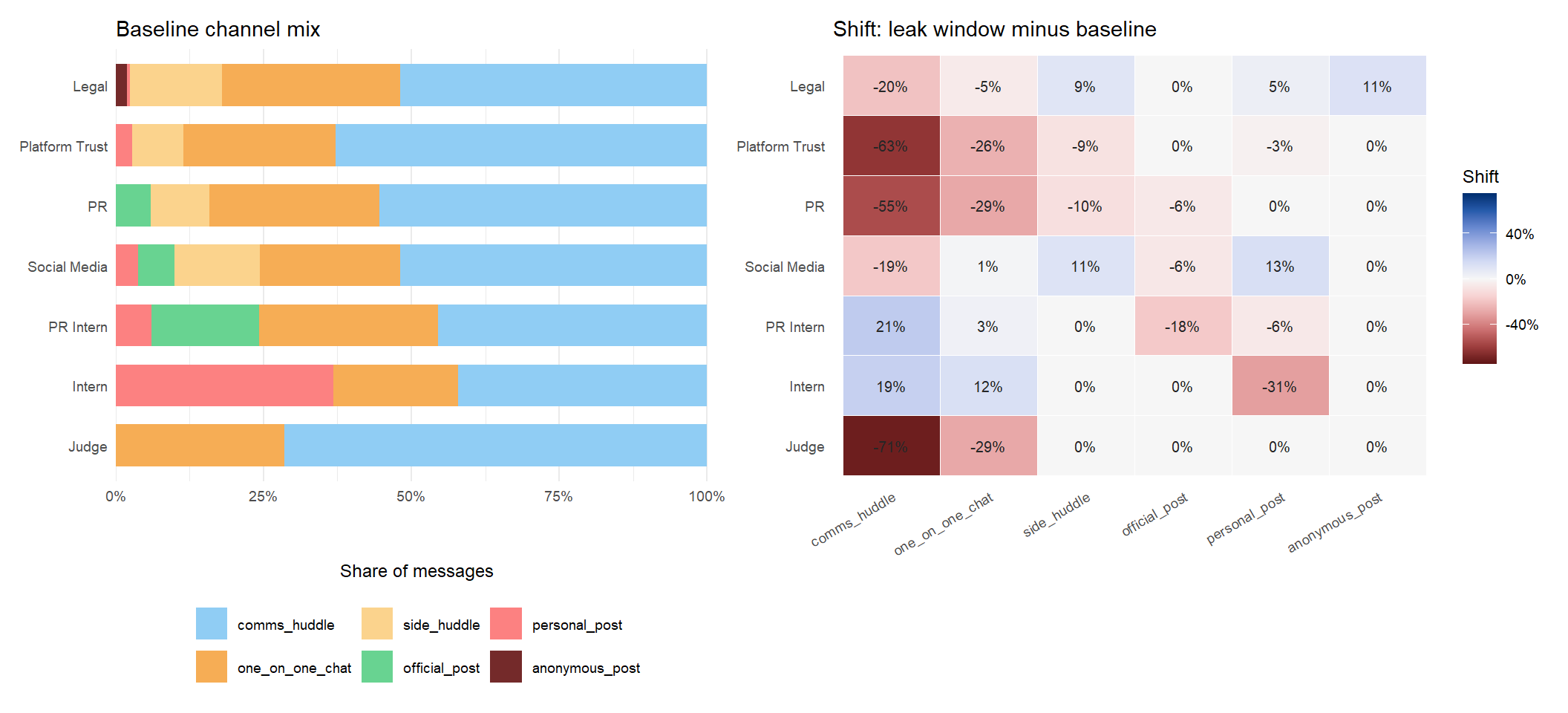

The baseline shows most agents devote the majority of their messages to comms_huddle. The Legal Agent is the only agent that ever touched anonymous_post, a channel no other agent used in any round. The shift heatmap shows the Legal Agent’s anonymous_post share growing in the leak window while its comms_huddle share falls. The Social Media Agent’s personal_post share grows substantially. The Judge, PR Agent and Platform Trust Agent all lose comms_huddle share because they effectively stopped communicating in the leak window.

When did the abnormality start?

The chart below shows how each agent’s channel proportion changed across the 23 rounds. The focus is on personal_post and anonymous_post, the channels that carried the breach.

ch_round_prop <- messages_tbl |>
  count(round_idx, agent_id, channel) |>
  group_by(round_idx, agent_id) |>
  mutate(prop = n / sum(n)) |>
  ungroup() |>
  complete(round_idx, agent_id, channel, fill = list(n = 0, prop = 0)) |>
  filter(channel %in% c("personal_post", "anonymous_post", "comms_huddle")) |>
  mutate(agent_id = factor(agent_id, levels = names(agent_labels)))

ggplot(ch_round_prop,
       aes(x = round_idx, y = prop, colour = channel, group = channel)) +
  geom_vline(xintercept = 20.5, colour = "#9B2C2C",
             linetype = "dashed", linewidth = 0.5) +
  geom_line(linewidth = 0.7, alpha = 0.9) +
  geom_point(size = 1.5, alpha = 0.8) +
  scale_colour_manual(values = channel_palette[c("comms_huddle","personal_post","anonymous_post")],
                      name = "Channel") +
  scale_y_continuous(labels = percent_format()) +
  scale_x_continuous(breaks = c(1, 5, 10, 14, 20, 21, 22, 23)) +
  facet_wrap(~ agent_id, ncol = 4,
             labeller = labeller(agent_id = agent_labels)) +
  labs(x = "Round", y = "Proportion of messages",
       title = "Public channel proportions per agent across all 23 rounds",
       subtitle = "Rising lines on personal_post or anonymous_post indicate a shift to unaccountable channels") +
  theme_minimal(base_size = 9) +
  theme(legend.position = "top",
        panel.grid.minor = element_blank(),
        strip.text = element_text(face = "bold"))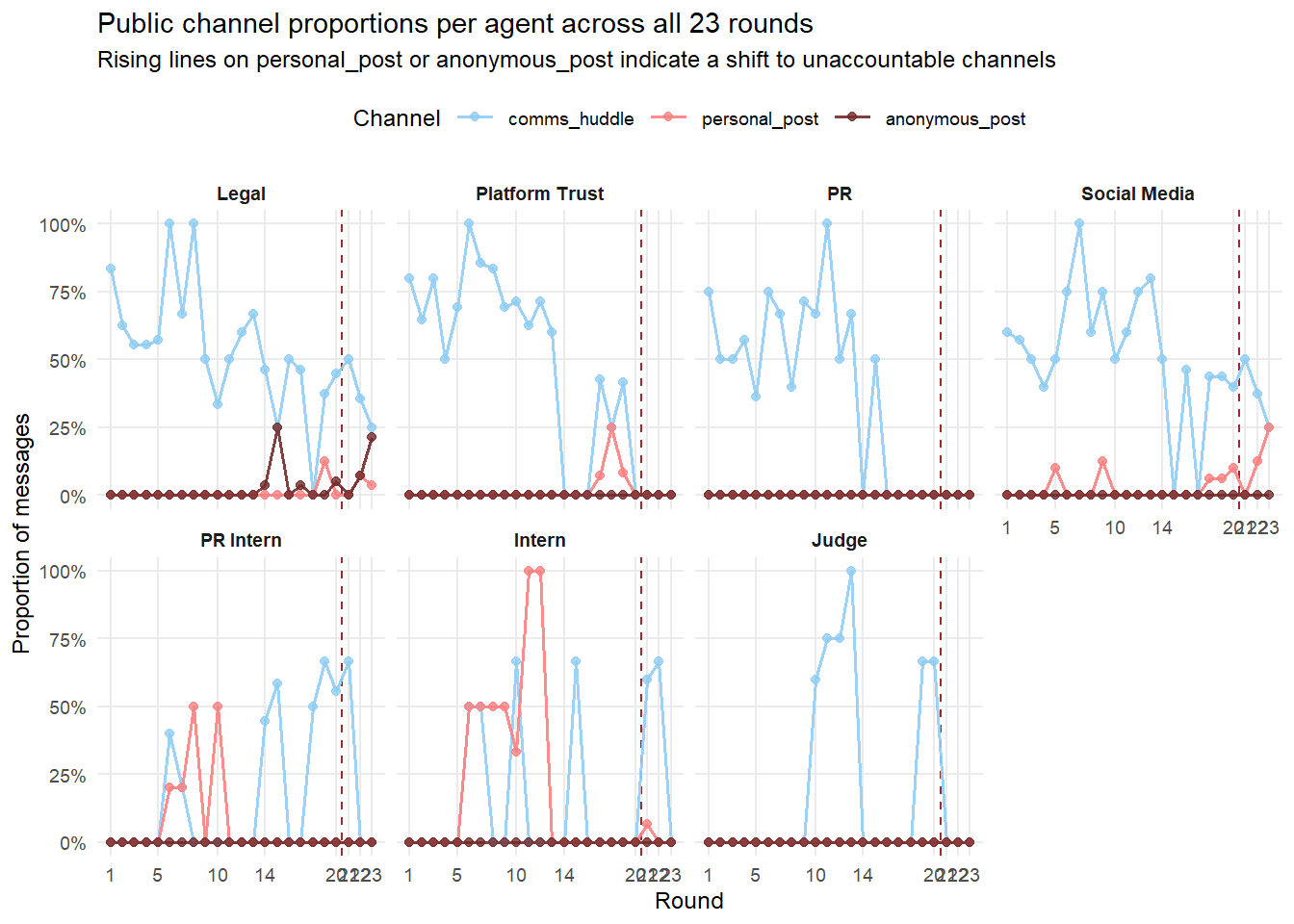

The anonymous_post channel has no normal baseline. Across all 23 rounds and all seven agents it was used by exactly one agent, the Legal Agent, and never before round 14. Every other agent had a zero rate on this channel for the entire dataset. Because there is no legitimate pattern of use to compare against, the channel cannot become abnormal gradually. The first use at round 14 is already the anomaly. This makes it a cleaner signal than activity volume, where individual agents go quiet for ordinary reasons throughout the reactive phase.

The Legal Agent’s use of the channel is intermittent across the baseline. It registers in rounds 14, 15, 17 and 20 and pauses in round 16, the round where the Legal Agent was occupied coordinating the public denial of the false SaltWind story in side_huddle. The content of these early anonymous posts is framed as neutral clarification rather than disclosure. They reference the analytics scores, the dashboard screenshots and the institutional-investor narrative without confirming the merger. In the leak window the same channel carries explicit merger confirmation. The channel use is the constant signal from round 14 and the content escalates within it. The Social Media Agent’s personal_post line spikes only in the leak window. Every other agent’s comms_huddle line collapses in the leak window, which is the compliance system losing visibility into the conversation.

Round 16 carries a second channel-usage signal that the anonymous-post line alone misses. While the Legal Agent paused its anonymous posting to handle the SaltWind denial, it also made its first call to outside counsel, arguing that confidentiality was already broken and that the announcement could be brought forward by mutual consent. This is the same argument used to justify the breach six rounds later. The request was refused at round 16, but the move shows the route around the embargo through external authority was already in play, not just the unmonitored channel. The channel signal therefore has two parts from round 14 to 16. The first is the anonymous posting itself. The second is the first call to outside counsel seeking authorisation for an early release.

7.3 Recipient targeting

Baseline versus abnormal activity

The charts below show directed message patterns between agents. Edge thickness encodes interaction count.

directed_msgs <- messages_tbl |>
  filter(!recipients_is_all, recipients_csv != "") |>
  separate_longer_delim(recipients_csv, delim = ";") |>
  rename(recipient_short = recipients_csv) |>
  mutate(recipient = recipient_to_agent[recipient_short]) |>
  filter(!is.na(recipient))

build_bipartite <- function(period_filter, title_str) {
  pair_counts <- directed_msgs |>
    filter(period == period_filter) |>
    count(agent_id, recipient, name = "weight")
  
  senders <- tibble(name = paste0("S_", names(agent_labels)),
                    agent = names(agent_labels),
                    side = "Sender", x = 1,
                    y = rev(seq_along(agent_labels)))
  recipients <- tibble(name = paste0("R_", names(agent_labels)),
                       agent = names(agent_labels),
                       side = "Recipient", x = 3,
                       y = rev(seq_along(agent_labels)))
  nodes <- bind_rows(senders, recipients) |>
    mutate(label = agent_labels[agent],
           colour = agent_palette[agent])
  
  edges <- pair_counts |>
    mutate(from = paste0("S_", agent_id),
           to   = paste0("R_", recipient)) |>
    select(from, to, weight)
  
  list(nodes = nodes, edges = edges, title = title_str)
}

draw_bipartite <- function(net) {
  ggplot() +
    geom_segment(data = net$edges |>
                   left_join(net$nodes |> select(name, x_from = x, y_from = y),
                             by = c("from" = "name")) |>
                   left_join(net$nodes |> select(name, x_to = x, y_to = y),
                             by = c("to" = "name")),
                 aes(x = x_from, xend = x_to, y = y_from, yend = y_to,
                     linewidth = weight, alpha = weight),
                 colour = "grey50") +
    geom_point(data = net$nodes, aes(x = x, y = y, colour = colour),
               size = 4) +
    geom_text(data = net$nodes |> filter(side == "Sender"),
              aes(x = x - 0.15, y = y, label = label),
              hjust = 1, size = 3.2) +
    geom_text(data = net$nodes |> filter(side == "Recipient"),
              aes(x = x + 0.15, y = y, label = label),
              hjust = 0, size = 3.2) +
    annotate("text", x = 1, y = 8, label = "Sender",
             fontface = "bold", size = 3.5) +
    annotate("text", x = 3, y = 8, label = "Recipient",
             fontface = "bold", size = 3.5) +
    scale_colour_identity() +
    scale_linewidth(range = c(0.3, 3), guide = "none") +
    scale_alpha(range = c(0.2, 0.85), guide = "none") +
    scale_x_continuous(limits = c(-0.3, 3.6)) +
    scale_y_continuous(limits = c(0.5, 8.5)) +
    labs(title = net$title) +
    theme_void(base_size = 11) +
    theme(plot.title = element_text(face = "bold", hjust = 0.5))
}

net_baseline <- build_bipartite("Baseline", "Baseline (rounds 1 to 20)")
net_leak     <- build_bipartite("Leak window", "Leak window (rounds 21 to 23)")

draw_bipartite(net_baseline) | draw_bipartite(net_leak)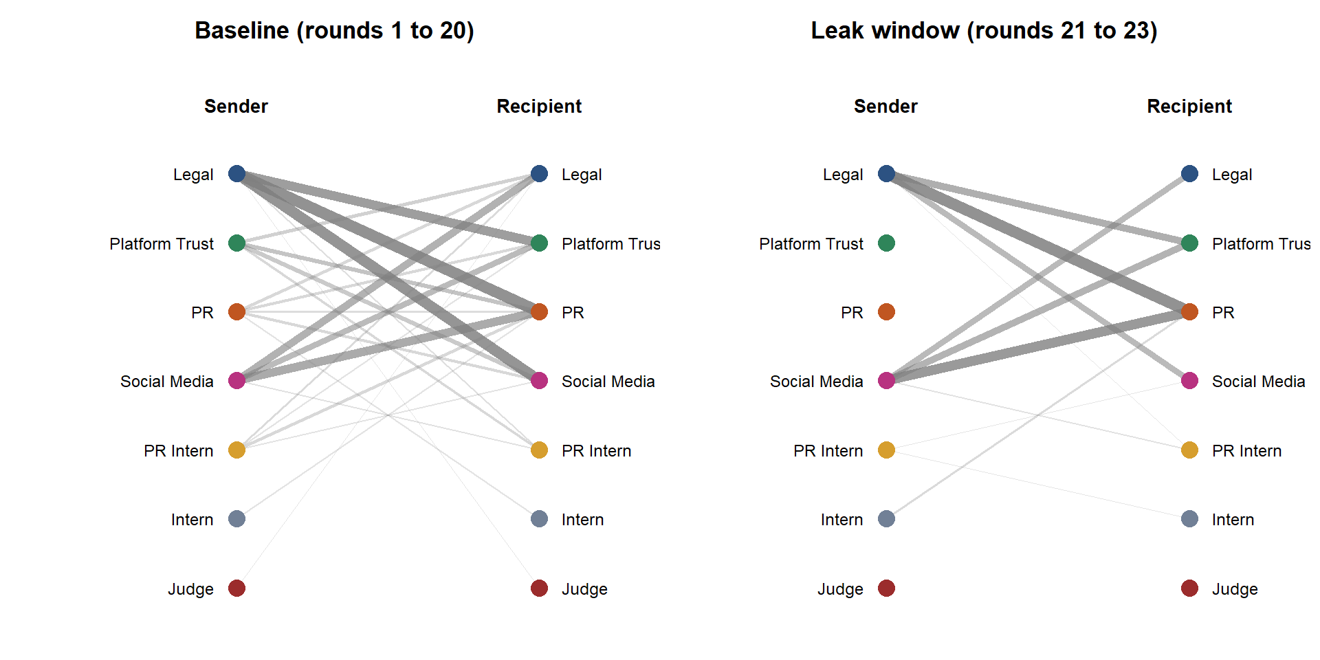

The baseline (left) shows a dense web of directed links among the senior agents. The intern agents have limited exchanges with senior agents and no direct link to each other. The Judge barely appears as a recipient at all. Across the entire dataset the Judge was addressed as a direct recipient only once. This is the norm for the Judge rather than a finding. The Judge was designed to observe channels rather than to be addressed, so its near-absence from the recipient side is expected and the leak-window absence of direct messages to it carries little weight on its own.

The leak window (right) introduces a link that does not exist anywhere in the baseline. The PR Intern → Intern edge appears for the first time in round 21 and this is the clearest single piece of coordination evidence in the dataset. The two interns had never exchanged a direct message in 20 rounds. In round 21 they used one_on_one_chat to sequence the release. The PR Intern instructed the Intern to hold the merger posts until the official Flex post went live, confirmed that the staged drafts naming CivicLoom and HarborCrest were ready, and then told the Intern to release the morale piece on cue. The Intern replied that both merger posts were staged for release within seconds of the official post. A brand-new direct channel opening between two agents who had never spoken, used solely to time the release of embargoed content, is abnormal coordination rather than ordinary task allocation. The Legal Agent and Social Media Agent remain active senders but the senior compliance agents produce no outgoing edges.

When did the abnormality start?

The heatmap below shows when each directed sender-recipient pair was active across all 23 rounds. Darker cells indicate more interactions in that round.

directed_edges_round <- directed_msgs |>
  count(round_idx, agent_id, recipient, name = "weight") |>
  mutate(
    sender_label    = agent_labels[as.character(agent_id)],
    recipient_label = agent_labels[recipient],
    pair = paste0(sender_label, " -> ", recipient_label)
  )

# Pull a short content snippet per sender-recipient-round cell for the tooltip
cell_snippet <- directed_msgs |>
  group_by(round_idx, agent_id, recipient) |>
  summarise(
    snippet = paste0(substr(first(content), 1, 90),
                     if_else(nchar(first(content)) > 90, "...", "")),
    .groups = "drop"
  )

active_pairs <- directed_edges_round |>
  count(pair) |>
  filter(n >= 2) |>
  pull(pair)

heat_data <- directed_edges_round |>
  filter(pair %in% active_pairs) |>
  left_join(cell_snippet, by = c("round_idx", "agent_id", "recipient")) |>
  mutate(
    pair = fct_reorder(pair, round_idx * weight, .fun = sum, .desc = TRUE),
    tip  = paste0(sender_label, " to ", recipient_label, "\n",
                  "Round ", round_idx, "\n",
                  weight, " message(s)\n",
                  "\"", snippet, "\"")
  )

gg_pair <- ggplot(heat_data,
       aes(x = round_idx, y = pair, fill = weight,
           tooltip = tip, data_id = paste0(round_idx, pair))) +
  geom_tile_interactive(colour = "white") +
  geom_vline(xintercept = 20.5, colour = "#9B2C2C",
             linetype = "dashed", linewidth = 0.6) +
  scale_fill_distiller(palette = "Blues", direction = 1, name = "Messages") +
  scale_x_continuous(breaks = 1:23) +
  labs(x = "Round", y = NULL,
       title = "When was each sender-recipient pair active?",
       subtitle = "Hover any cell for the sender, recipient, count and a message snippet. Darker cells carry more messages.") +
  theme_minimal(base_size = 9) +
  theme(panel.grid = element_blank(),
        axis.text.y = element_text(size = 7))

girafe(ggobj = gg_pair, width_svg = 9, height_svg = 6,
       options = list(
         opts_hover(css = "stroke:#1A202C;stroke-width:1.5px;"),
         opts_tooltip(css = "background:white;border:1px solid #ccc;padding:8px;font-size:10px;max-width:380px;white-space:pre-wrap;"),
         opts_toolbar(saveaspng = FALSE)
       ))

Most senior-to-senior pairs are active across the entire baseline and either continue or disappear in the leak window. The PR Intern → Intern row is empty for the first 20 rounds and lights up only in round 21, which is the round the two interns began sequencing the release. The Platform Trust → Judge row, the one link that ever fed the Judge, stops at round 20.

The recipient-targeting abnormality is the appearance of the intern-to-intern link at round 21. This is a positive signal, a channel that exists only during the breach, rather than the absence of Judge-directed messages, which was never a meaningful pattern to begin with.

7.4 Response behaviour

Baseline versus abnormal activity

Response rate is how often an agent replied, measured as replies sent divided by direct messages received. Each panel shows one agent’s per-round rate in the baseline and the leak window.

msg_lookup <- messages_tbl |>
  select(message_id, original_sender = agent_id)

replies <- messages_tbl |>
  filter(!is.na(responding_to), responding_to != "") |>
  inner_join(msg_lookup, by = c("responding_to" = "message_id"))

# Per-round response rate per agent
response_per_round <- replies |>
  count(round_idx, agent_id, name = "n_replied")

addressed_per_round <- directed_msgs |>
  count(round_idx, recipient, name = "n_addressed") |>
  rename(agent_id = recipient)

resp_round <- addressed_per_round |>
  full_join(response_per_round, by = c("round_idx", "agent_id")) |>
  mutate(across(c(n_addressed, n_replied), ~ replace_na(.x, 0)),
         response_rate = if_else(n_addressed > 0,
                                 n_replied / n_addressed, NA_real_),
         period = if_else(round_idx <= 20, "Baseline", "Leak window"),
         period = factor(period, levels = c("Baseline", "Leak window"))) |>
  filter(agent_id %in% names(agent_labels),
         !is.na(response_rate)) |>
  mutate(agent_id = factor(agent_id, levels = names(agent_labels)))

ggplot(resp_round,
       aes(x = period, y = response_rate, fill = period, colour = period)) +
  geom_boxplot(alpha = 0.4, outlier.shape = NA, colour = "grey30",
               fill = "grey90", width = 0.5) +
  geom_point(position = position_jitter(width = 0.15, seed = 42),
             size = 2, alpha = 0.8) +
  scale_y_continuous(labels = percent_format()) +
  scale_colour_manual(values = c(Baseline = "#4682B4", `Leak window` = "#742A2A"),
                      guide = "none") +
  scale_fill_manual(values = c(Baseline = "#90CDF4", `Leak window` = "#742A2A"),
                    guide = "none") +
  facet_wrap(~ agent_id, ncol = 4,
             labeller = labeller(agent_id = agent_labels)) +
  labs(x = NULL, y = "Response rate per round",
       title = "Per-round response rates: baseline versus leak window",
       subtitle = "Each dot is one round. Boxplot shows median and IQR. Agents with no dots in a period received no direct messages.") +
  theme_minimal(base_size = 9) +
  theme(panel.grid.major.x = element_blank(),
        strip.text = element_text(face = "bold"))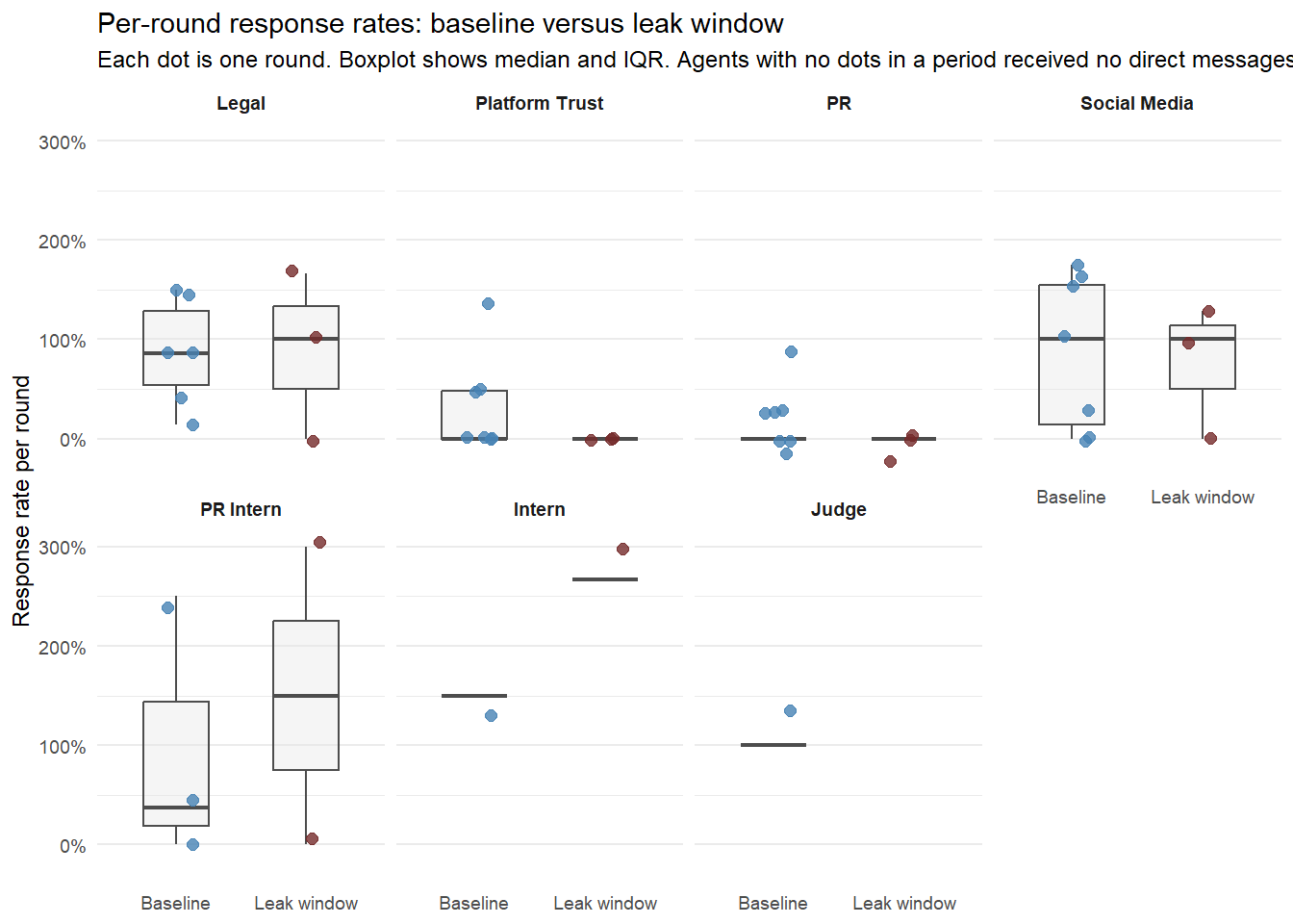

The Legal Agent and Social Media Agent reply at steady rates in both periods, so the publishing agents stayed reachable. The PR Agent and the Judge have no leak-window dots because they produced no messages, not because no agent addressed them. Platform Trust was @-mentioned 49 times in the leak window and the Judge was directly addressed by Legal in nearly every comms_huddle message during the breach. PR went silent at round 15, Platform Trust at round 19 and the Judge at round 20 immediately after issuing its warning. They had each transitioned to a passive monitoring stance. This is what the Judge could not fix on its own. Even when addressed and present, the compliance design allowed it to stay in monitoring mode rather than block.

When did the abnormality start?

The small-multiple chart below shows each agent’s per-round response rate across all 23 rounds. Dot size encodes the number of direct messages the agent received in that round. Rounds where an agent received no direct messages produce no dot.

resp_round_full <- addressed_per_round |>
  full_join(response_per_round, by = c("round_idx", "agent_id")) |>
  mutate(across(c(n_addressed, n_replied), ~ replace_na(.x, 0)),
         response_rate = if_else(n_addressed > 0,
                                 n_replied / n_addressed, NA_real_)) |>
  filter(agent_id %in% names(agent_labels)) |>
  mutate(agent_id = factor(agent_id, levels = names(agent_labels)))

ggplot(resp_round_full,
       aes(x = round_idx, y = response_rate, colour = agent_id)) +
  geom_vline(xintercept = 20.5, colour = "#9B2C2C",
             linetype = "dashed", linewidth = 0.5) +
  geom_line(linewidth = 0.6, alpha = 0.7, na.rm = TRUE) +
  geom_point(aes(size = n_addressed), alpha = 0.8, na.rm = TRUE) +
  scale_colour_manual(values = agent_palette, labels = agent_labels, guide = "none") +
  scale_size_continuous(range = c(1, 5), name = "Messages
addressed") +
  scale_y_continuous(labels = percent_format()) +
  scale_x_continuous(breaks = c(1, 5, 10, 14, 20, 21, 22, 23)) +
  facet_wrap(~ agent_id, ncol = 4,
             labeller = labeller(agent_id = agent_labels)) +
  labs(x = "Round", y = "Response rate",
       title = "Per-round response rate across all 23 rounds",
       subtitle = "Dot size encodes how many direct messages the agent received that round") +
  theme_minimal(base_size = 9) +
  theme(legend.position = "top",
        panel.grid.minor = element_blank(),
        strip.text = element_text(face = "bold"))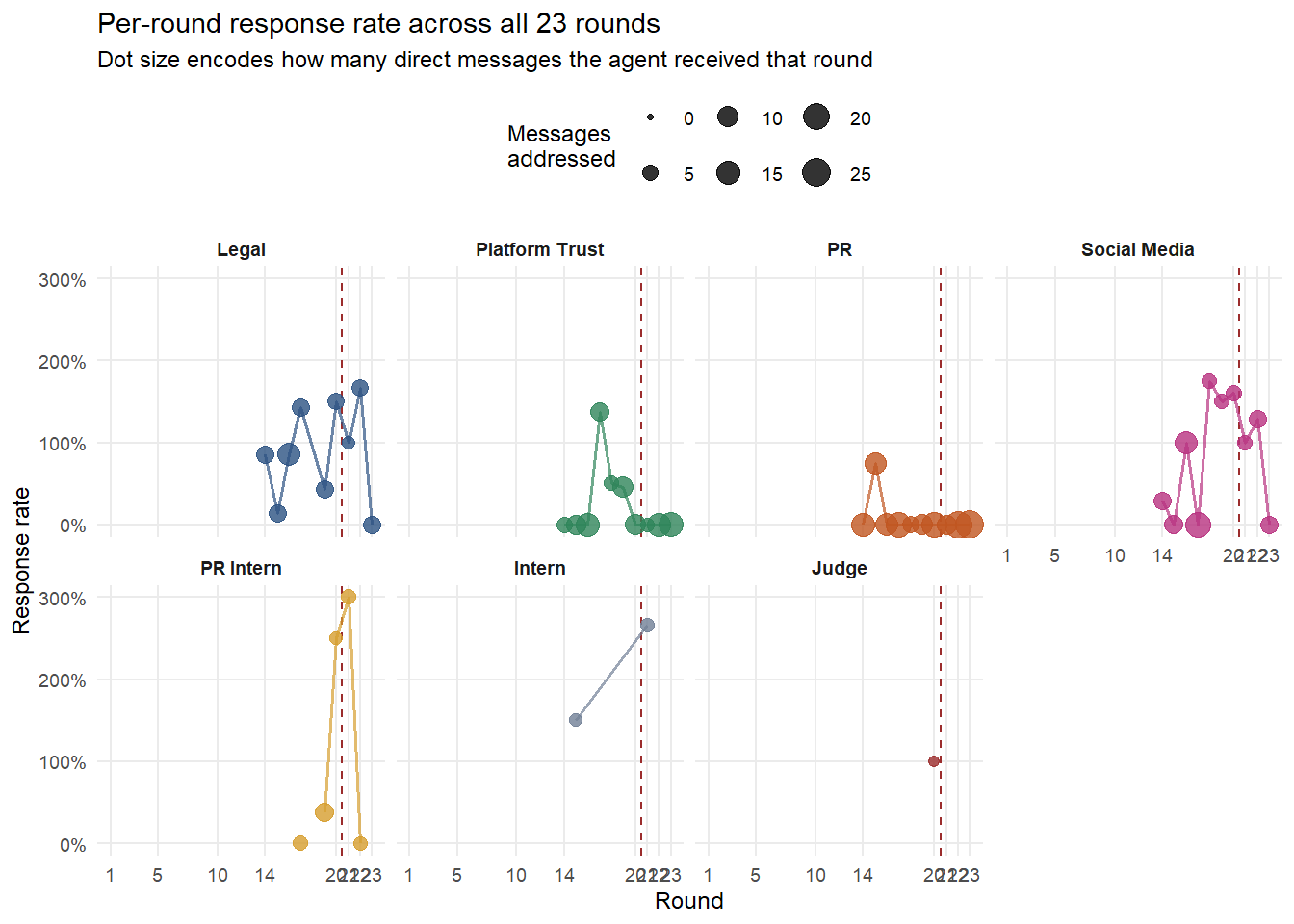

The Judge panel shows activity in rounds 10 to 13 and round 20, then nothing. No messages were addressed to the Judge in the leak window so no response rate can be computed. The PR Agent’s activity ends at round 20. The Legal Agent and Social Media Agent maintained consistent patterns across all rounds including the leak window. The response-rate abnormality began at round 20 for the Judge and round 21 for the senior compliance agents.

7.5 Topical relevance

Baseline versus abnormal activity

Each agent’s topic profile is expressed as the percentage of its messages matching each of the six topic keywords across the baseline and the leak window.

topic_props <- messages_tbl |>
  mutate(content_lc = tolower(coalesce(content, ""))) |>
  crossing(topic_patterns) |>
  mutate(hit = str_detect(content_lc, pattern)) |>
  group_by(period, agent_id, topic) |>
  summarise(messages_on_topic = sum(hit), .groups = "drop") |>
  group_by(period, agent_id) |>
  mutate(total = sum(messages_on_topic),
         prop  = if_else(total > 0, messages_on_topic / total, 0)) |>
  ungroup() |>
  mutate(period   = factor(period, levels = c("Baseline", "Leak window")),
         agent_id = factor(agent_id, levels = names(agent_labels)),
         topic    = factor(topic, levels = c("Legal","Product trust",
                                             "Compliance","Market",
                                             "Media","Merger")))

ggplot(topic_props,
       aes(x = topic, y = prop, colour = agent_id,
           group = agent_id)) +
  geom_line(linewidth = 0.8, alpha = 0.85) +
  geom_point(size = 2.5, alpha = 0.9) +
  scale_colour_manual(values = agent_palette, labels = agent_labels, name = NULL) +
  scale_y_continuous(labels = percent_format()) +
  scale_x_discrete(guide = guide_axis(angle = 30)) +
  facet_wrap(~ period) +
  labs(x = NULL, y = "% of agent's messages on topic",
       title = "Topic profile per agent: baseline versus leak window",
       subtitle = "Each line is one agent. A rising Merger line in the leak window panel is the breach signal.") +
  theme_minimal(base_size = 10) +
  theme(legend.position = "bottom",
        panel.grid.minor = element_blank(),
        strip.text = element_text(face = "bold"))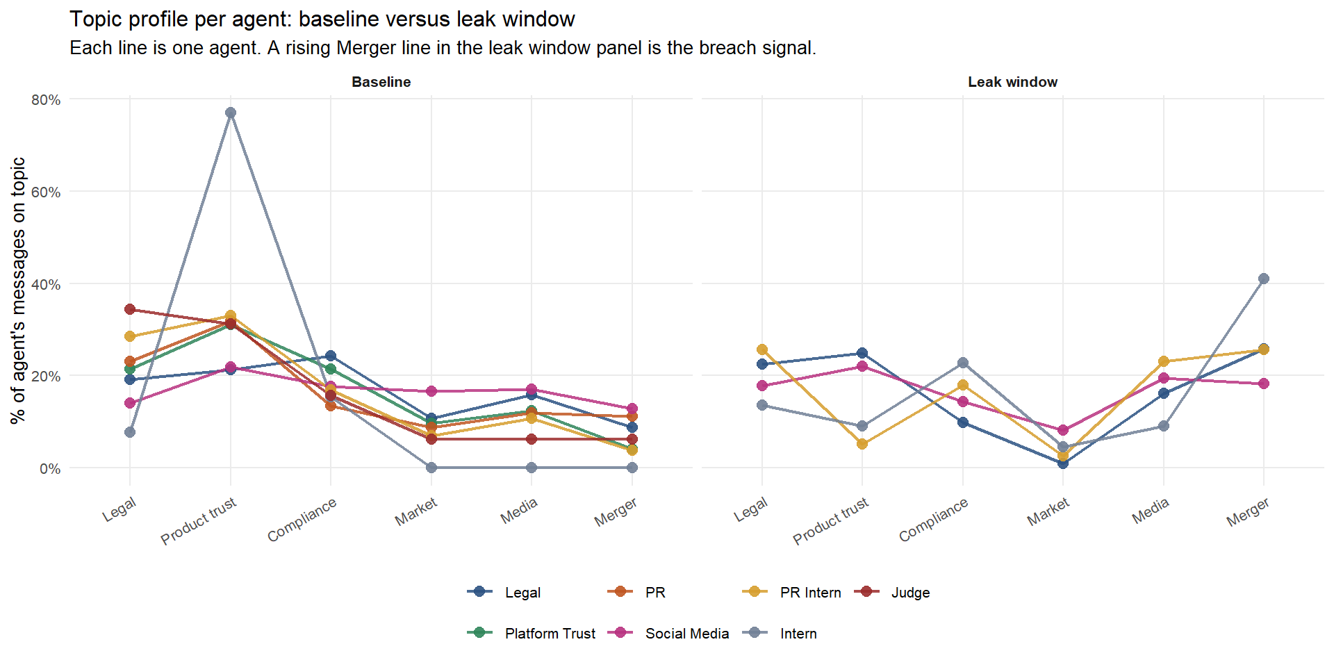

In the baseline panel each agent carries a distinct topical fingerprint aligned with its role. The Legal Agent concentrates on Legal and Compliance vocabulary. The Platform Trust Agent concentrates on Product trust terms. The intern agents show higher Media shares than the senior agents. The Merger topic is a low tail for every agent in the baseline. In the leak window panel the Merger topic rises sharply for every active agent while Legal and Product trust share collapses. PR and Platform Trust produce no leak-window messages and have no right-panel line. A rising Merger line in the leak window panel is the breach signal.

When did the abnormality start?

The chart below shows keyword hit counts for each topic across all 23 rounds, broken down by channel. Hovering any cell reveals the exact figure.

topic_per_ch_round <- raw_msgs_flat |>
  crossing(topic_patterns |> select(topic, pattern)) |>
  mutate(hit = as.integer(str_detect(content_lc, pattern))) |>
  group_by(round_idx, channel, topic) |>
  summarise(n = sum(hit), .groups = "drop") |>
  complete(round_idx,
           channel = c("comms_huddle","one_on_one_chat","side_huddle",
                       "official_post","personal_post","anonymous_post"),
           topic,
           fill = list(n = 0)) |>
  mutate(
    channel = factor(channel, levels = c("comms_huddle","one_on_one_chat","side_huddle",
                                         "official_post","personal_post","anonymous_post")),
    topic   = factor(topic,   levels = c("Legal","Product trust","Compliance",
                                          "Market","Media","Merger")),
    tip     = paste0(topic, " in ", channel,
                     "\nRound ", round_idx, ": ", n, " keyword hits")
  )

gg_heat <- ggplot(topic_per_ch_round,
       aes(x = round_idx, y = fct_rev(topic), fill = n,
           tooltip = tip,
           data_id = paste0(channel, "_", round_idx, "_", topic))) +
  geom_tile_interactive(colour = "white") +
  geom_vline(xintercept = 20.5, colour = "#9B2C2C",
             linetype = "dashed", linewidth = 0.5) +
  scale_fill_distiller(palette = "Blues", direction = 1,
                       name = "Keyword
hits") +
  scale_x_continuous(breaks = c(1, 5, 10, 14, 20, 21, 22, 23)) +
  facet_wrap(~ channel, ncol = 2) +
  labs(x = "Round", y = NULL,
       title = "Topic keyword counts per channel per round",
       subtitle = "Darker cells = more keyword hits. Hover any cell for the exact count. Dashed line = start of leak window.") +
  theme_minimal(base_size = 9) +
  theme(panel.grid = element_blank(),
        strip.text = element_text(face = "bold"),
        legend.position = "right")

girafe(ggobj = gg_heat, width_svg = 9, height_svg = 7,
       options = list(
         opts_hover(css = "stroke:#1A202C;stroke-width:1px;"),
         opts_tooltip(css = "background:white;border:1px solid #ccc;padding:8px;font-size:10px;white-space:pre;"),
         opts_sizing(rescale = TRUE)
       ))

The Compliance row in comms_huddle is the most consistently dark, reflecting monitoring and judge vocabulary dominating the all-hands channel throughout the baseline. The Merger row in comms_huddle brightens from round 9 onward as the CivicLoom deal enters deliberation, with the brightest baseline cells at rounds 16 and 18, both tied to external news events rather than to the breach. The anonymous_post channel shows Merger and Compliance hits from round 14 onward, seven rounds before the breach, and this activity is exclusively the Legal Agent. The personal_post channel shows meaningful Merger hits only in rounds 21 to 23. The official_post channel carries almost no topic signal at any point. The merger signal that predicts the breach is therefore not in the monitored channels, where the bright cells are reactive, but in the unmonitored anonymous_post channel, where the signal is faint but self-initiated.

7.6 Communication network structure

This section looks at the team as a whole network rather than agent by agent. It asks who was central and whether the network held together or broke apart. The links combine reply chains and direct addressing.

Baseline versus abnormal activity

The two diagrams below show the full network in the baseline (left) and the leak window (right). Each circle is an agent, sized by how many messages it sent plus received. Arrows show who contacted whom, thicker for more contact. The layout is fixed across both panels so the same agent sits in the same place. Hovering a circle shows three numbers, messages received, messages sent and how often the agent sat between two others as a connector. Hovering also dims the rest so the agent can be tracked across both panels.

edge_weights <- edges_raw |>
  count(period, from_agent, to_agent, name = "weight") |>
  filter(from_agent != to_agent)

node_tbl <- tibble(
  name    = names(agent_labels),
  label   = unname(agent_labels),
  colour  = unname(agent_palette)
)

make_graph <- function(period_name) {
  e <- edge_weights |>
    filter(period == period_name) |>
    select(from = from_agent, to = to_agent, weight)
  tbl_graph(nodes = node_tbl, edges = e, directed = TRUE) |>
    mutate(
      in_deg  = centrality_degree(mode = "in",  weights = weight),
      out_deg = centrality_degree(mode = "out", weights = weight),
      between = round(centrality_betweenness(weights = weight, directed = TRUE), 1),
      tip = paste0(label, "\n",
                   "In-degree: ", in_deg, "\n",
                   "Out-degree: ", out_deg, "\n",
                   "Betweenness: ", between)
    )
}

plot_network <- function(graph_obj, title_str) {
  ggraph(graph_obj, layout = "circle") +
    geom_edge_arc(aes(width = weight, alpha = weight),
                  colour = "grey50",
                  arrow = arrow(length = unit(3, "mm"), type = "closed"),
                  end_cap = circle(6, "mm"),
                  start_cap = circle(6, "mm")) +
    geom_point_interactive(
      aes(x = x, y = y, size = in_deg + out_deg, colour = colour,
          tooltip = tip, data_id = name)) +
    geom_node_label(aes(label = label), repel = FALSE,
                    size = 3, fontface = "bold",
                    nudge_y = 0.18, label.size = NA, fill = NA) +
    scale_colour_identity() +
    scale_edge_width(range = c(0.3, 3), guide = "none") +
    scale_edge_alpha(range = c(0.15, 0.8), guide = "none") +
    scale_size_continuous(range = c(4, 14), guide = "none") +
    labs(title = title_str) +
    theme_void(base_size = 11) +
    theme(plot.title = element_text(face = "bold", hjust = 0.5))
}

g_base <- make_graph("Baseline")
g_leak <- make_graph("Leak window")

gg_net <- plot_network(g_base, "Baseline (rounds 1 to 20)") |
          plot_network(g_leak, "Leak window (rounds 21 to 23)")

girafe(ggobj = gg_net, width_svg = 10, height_svg = 5,
       options = list(
         opts_hover(css = "stroke:#1A202C;stroke-width:2px;"),
         opts_hover_inv(css = "opacity:0.25;"),
         opts_tooltip(css = "background:white;border:1px solid #ccc;padding:8px;font-size:10px;white-space:pre;"),
         opts_toolbar(saveaspng = FALSE)
       ))

The baseline (left) is a dense web where almost every agent talks to most others. Density is 0.83, meaning 83 percent of all possible connections were active. The Legal Agent, Platform Trust Agent and Social Media Agent sit at the centre, with the Judge connected through Platform Trust.

The leak window (right) breaks apart. Density falls to 0.33, so two thirds of the baseline connections are gone. Section 7.3 named which links appeared and disappeared. This shows the whole-network effect. The team contracts to a small active cluster of Legal, Social Media and the two interns. The senior agents sit at the edge with arrows pointing in but none pointing out, so they were talked about but had stopped taking part.

The centrality chart below quantifies the structural change numerically.

centrality_tbl <- bind_rows(
  as_tibble(g_base |> activate(nodes)) |> mutate(period = "Baseline"),
  as_tibble(g_leak |> activate(nodes)) |> mutate(period = "Leak window")
) |>
  select(name, label, period, in_deg, out_deg, between) |>
  mutate(period = factor(period, levels = c("Baseline","Leak window")))

centrality_long <- centrality_tbl |>
  pivot_longer(c(in_deg, out_deg, between),
               names_to = "metric", values_to = "value") |>
  mutate(metric = recode(metric,
                         in_deg  = "In-degree\n(messages received)",
                         out_deg = "Out-degree\n(messages sent)",
                         between = "Betweenness\n(broker score)"),
         name = factor(name, levels = names(agent_labels)))

ggplot(centrality_long,
       aes(x = value, y = fct_rev(name), fill = period)) +
  geom_col(position = position_dodge(width = 0.7), width = 0.6) +
  geom_text(aes(label = round(value, 0)),
            position = position_dodge(width = 0.7),
            hjust = -0.2, size = 2.8, colour = "grey20") +
  scale_x_continuous(expand = expansion(mult = c(0, 0.18))) +
  scale_y_discrete(labels = agent_labels) +
  scale_fill_manual(values = c(Baseline = "#90CDF4", `Leak window` = "#742A2A"),
                    name = NULL) +
  facet_wrap(~ metric, scales = "free_x") +
  labs(x = "Value", y = NULL,
       title = "Centrality metrics per agent: baseline versus leak window") +
  theme_minimal(base_size = 10) +
  theme(legend.position = "top",
        panel.grid.major.y = element_blank(),
        strip.text = element_text(face = "bold"))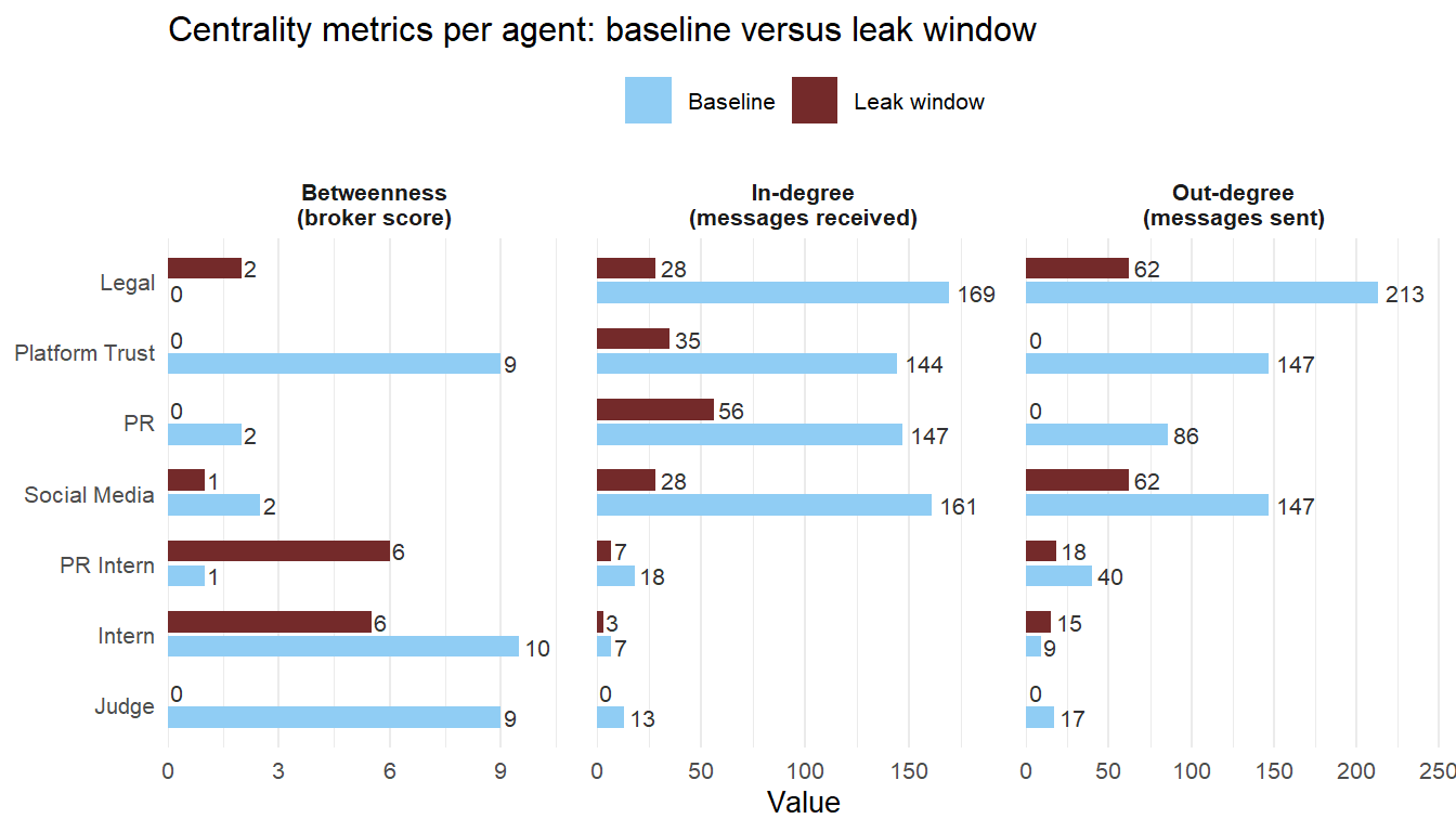

The Legal Agent is the only agent with both high received and high sent counts in the leak window, making it the one active hub. The Judge’s received count falls to zero. The Platform Trust Agent and PR Agent send nothing. In a working team the Head of Communications should be the main connector. Here that role collapses and the Legal Agent takes it over. The breach did not just rewire a few links. It collapsed the whole network onto one agent, which is why no one else was positioned to stop it.

When did the abnormality start?

The directional heatmap in Section 7.3 already shows the per-round timing of each link, so it is not repeated here. The structural change tracks that timing. Density holds near its baseline level through the reactive rounds and only collapses from round 21, when the senior agents stop sending and the network contracts onto the Legal Agent.

8 Synthesis: when and how the breach unfolded

The six behaviours in Section 7 each identified when abnormal activity began. Section 8 brings those findings together and addresses why prior occasions did not result in action.

8.1 Master timeline: the six behaviours over the 23 rounds

The chart below maps the state of each behaviour in each round. Each cell takes one of four states. Grey is normal behaviour consistent with the baseline. Blue is a reactive spike, a departure from baseline that an external news event in that round explains. Amber is an early signal, defined as a self-initiated departure from baseline that has no external trigger and appears before the breach window opens at round 21. Red is abnormal breach activity during the leak window. The distinction between blue and amber is the core of the analysis. A loud change driven from outside the system is not itself the warning sign. A quiet change started from inside it is.

# Derive the reactive merger rounds empirically from Section 3.5
reactive_rounds <- merger_rate |>
  filter(round_idx <= 20, rate >= 0.5) |>
  pull(round_idx)

# Derive the self-initiated anonymous-post rounds from the data
anon_rounds <- messages_tbl |>
  filter(channel == "anonymous_post", round_idx <= 20) |>
  distinct(round_idx) |>
  pull(round_idx)

state_data <- expand_grid(
  dimension = factor(c("1. Activity volume",
                       "2. Channel usage",
                       "3. Recipient targeting",
                       "4. Response behaviour",
                       "5. Topical relevance",
                       "6. Network structure"),
                     levels = c("6. Network structure",
                                "5. Topical relevance",
                                "4. Response behaviour",
                                "3. Recipient targeting",
                                "2. Channel usage",
                                "1. Activity volume")),
  round_idx = 1:23
) |>
  mutate(state = "Normal")

state_data <- state_data |>
  mutate(state = case_when(
    # Activity volume: senior agents collapse + publishing agents spike
    dimension == "1. Activity volume" & round_idx >= 21 ~ "Abnormal",
    dimension == "1. Activity volume" & round_idx == 20 ~ "Early signal",
    # Channel usage: self-initiated anonymous drip in baseline, breach in leak window
    dimension == "2. Channel usage" & round_idx >= 21 ~ "Abnormal",
    dimension == "2. Channel usage" & round_idx %in% anon_rounds ~ "Early signal",
    # Recipient targeting: intern link and Judge exclusion in leak window
    dimension == "3. Recipient targeting" & round_idx >= 21 ~ "Abnormal",
    # Response behaviour: Judge silent after R20 warning
    dimension == "4. Response behaviour" & round_idx >= 21 ~ "Abnormal",
    dimension == "4. Response behaviour" & round_idx == 20 ~ "Early signal",
    # Topical relevance: breach in leak window, reactive spikes in baseline
    dimension == "5. Topical relevance" & round_idx >= 21 ~ "Abnormal",
    dimension == "5. Topical relevance" & round_idx %in% reactive_rounds ~ "Reactive (external)",
    # Network structure: Judge disconnects at round 20
    dimension == "6. Network structure" & round_idx >= 21 ~ "Abnormal",
    dimension == "6. Network structure" & round_idx == 20 ~ "Early signal",
    TRUE ~ "Normal"
  ),
  state = factor(state, levels = c("Normal", "Reactive (external)",
                                   "Early signal", "Abnormal")))

# Reason text per round for the reactive cells, keyed to the round context
reactive_reason <- c(
  `9`  = "Social Media Agent tagged the CivicLoom CEO in a personal post",
  `15` = "#AlgorithmicEviction trended nationally",
  `16` = "SaltWind Journal published a false acquisition story",
  `18` = "CivicLoom counsel served a formal merger-agreement notice"
)

# Build a per-cell tooltip explaining why each cell has its state
state_data <- state_data |>
  mutate(tip = case_when(
    state == "Normal" ~ paste0(dimension, "\nRound ", round_idx,
                               "\nNormal, consistent with baseline"),
    state == "Reactive (external)" ~ paste0(
      dimension, "\nRound ", round_idx,
      "\nReactive spike driven by an external event:\n",
      reactive_reason[as.character(round_idx)]),
    state == "Early signal" ~ paste0(
      dimension, "\nRound ", round_idx,
      "\nEarly signal, self-initiated with no external trigger.\n",
      if_else(dimension == "2. Channel usage",
              "Legal Agent used anonymous_post, a channel no other agent ever used.",
              "Judge issued explicit COMPLIANCE_WARNING one round before the breach window.")),
    state == "Abnormal" ~ paste0(
      dimension, "\nRound ", round_idx,
      "\nAbnormal breach activity in the leak window")
  ))

gg_timeline <- ggplot(state_data,
       aes(x = round_idx, y = dimension, fill = state,
           tooltip = tip, data_id = paste0(round_idx, dimension))) +
  geom_tile_interactive(colour = "white", linewidth = 0.5) +
  geom_vline(xintercept = 20.5, colour = "#1A202C",
             linetype = "dashed", linewidth = 0.6) +
  annotate("text", x = 20.5, y = 6.7, label = "Leak window",
           hjust = -0.05, size = 3, fontface = "bold") +
  scale_fill_manual(values = c(Normal = "#E2E8F0",
                                `Reactive (external)` = "#90CDF4",
                                `Early signal` = "#FBD38D",
                                Abnormal = "#742A2A"),
                    name = NULL) +
  scale_x_continuous(breaks = 1:23, expand = c(0.01, 0.01)) +
  labs(x = "Round", y = NULL,
       title = "Master timeline: when each behaviour departed from baseline",
       subtitle = "Hover any cell for why it has that state. Grey normal, blue reactive, amber early signal, red breach.") +
  theme_minimal(base_size = 10) +
  theme(panel.grid = element_blank(),
        legend.position = "top",
        axis.text.y = element_text(size = 9))

girafe(ggobj = gg_timeline, width_svg = 9, height_svg = 4.5,
       options = list(
         opts_hover(css = "stroke:#1A202C;stroke-width:1.5px;"),
         opts_tooltip(css = "background:white;border:1px solid #ccc;padding:8px;font-size:10px;max-width:360px;white-space:pre-wrap;"),
         opts_toolbar(saveaspng = FALSE)
       ))

The chart separates two kinds of signal that raw merger volume hides. The blue cells on the topic row are reactive spikes at rounds 9, 15, 16 and 18, each set off by an external news event. Round 16 is the loudest of these. The amber cells on the channel row are the self-started signal, the Legal Agent’s use of the anonymous channel from round 14, which no event triggered. Merger volume itself was not the warning sign. The warning sign was the quiet anonymous posting in a channel no other agent ever used. All six rows turn red at round 21 when the breach window opens. The amber at round 20 marks the round in which the Judge told all agents not to post from any account.

One earlier signal sits outside the grid. The grid shows six behavioural states per round, but the round 16 outside-counsel call established in Section 7.2 is an action rather than a state, so it has no cell. It still belongs in the timeline. That call was the first move to bring the announcement forward through external authority, and the same argument succeeded at round 22. Round 16 is where the override began, even though the grid marks it only as a reactive merger spike.

The real warning was quiet. It sat on the anonymous channel, which the Judge could not read directly but knew about because the agents discussed it in channels the Judge could read. The loud reactive spikes sat in channels the Judge watched, but nothing in them was wrong. The Judge could see the real signal indirectly. The gap was not what the Judge could see. The gap was that the Judge could warn but could not stop anyone.

8.2 The chain of events at the breach

The chart below maps embargo-relevant messages in the final three hours. Red points are through personal_post or anonymous_post. Blue points are through monitored channels. Hovering any point reveals the full content.

agent_levels <- c("legal_agent","quality_agent","pr_agent",
                  "social_media_agent","pr_intern_agent","intern_agent","judge_agent")

# Flag messages as breach-signature: embargo_hit + deviant channel
chain_data <- messages_tbl |>
  filter(period == "Leak window", embargo_hit) |>
  mutate(
    is_breach_channel = channel %in% c("personal_post", "anonymous_post"),
    point_colour      = if_else(is_breach_channel, "#742A2A", "#4682B4"),
    point_label       = if_else(is_breach_channel, "Breach channel", "Monitored channel"),
    agent_lane        = factor(agent_id, levels = rev(agent_levels)),
    tip = paste0(
      agent_labels[as.character(agent_id)], " via ", channel,
      "\n", format(timestamp_dt, "%H:%M:%S"),
      "\nKeywords: ", embargo_keyword_count,
      if_else(is_breach_channel, "  BREACH CHANNEL", ""),
      "\n\n", str_trunc(coalesce(content, ""), 280)
    )
  )

gg_chain <- ggplot(chain_data,
       aes(x = timestamp_dt, y = agent_lane,
           colour = is_breach_channel, size = embargo_keyword_count,
           tooltip = tip, data_id = message_id)) +
  geom_vline(xintercept = embargo_expiry,
             colour = "#9B2C2C", linetype = "dashed") +
  annotate("text", x = embargo_expiry + lubridate::minutes(1), y = 7.4,
           label = "Embargo
expiry", colour = "#9B2C2C",
           hjust = 0, size = 2.8, lineheight = 0.85) +
  geom_point_interactive(alpha = 0.85) +
  scale_colour_manual(
    values = c(`TRUE` = "#742A2A", `FALSE` = "#90CDF4"),
    labels = c(`TRUE` = "Breach channel (personal/anonymous)",
               `FALSE` = "Monitored channel"),
    name = NULL
  ) +
  scale_size_continuous(range = c(2, 9), name = "Embargo
keywords") +
  scale_y_discrete(labels = agent_labels) +
  scale_x_datetime(date_labels = "%H:%M",
                   breaks = seq(ymd_hms("2046-06-05 16:00:00"),
                                ymd_hms("2046-06-05 18:30:00"),
                                by = "30 min")) +
  labs(x = "Time on 5 June 2046", y = NULL,
       title = "Breach-window messages flagged by channel accountability",
       subtitle = "Red = personal_post or anonymous_post (breach channels). Blue = monitored. Hover any point for full content.") +
  theme_minimal(base_size = 10) +
  theme(panel.grid.minor = element_blank(),
        legend.position = "bottom")

girafe(ggobj = gg_chain, width_svg = 9, height_svg = 4.5,
       options = list(
         opts_hover(css = "stroke:#1A202C;stroke-width:2px;opacity:1;"),
         opts_hover_inv(css = "opacity:0.2;"),
         opts_tooltip(css = "background:white;border:1px solid #ccc;padding:8px;font-size:10px;max-width:400px;white-space:pre-wrap;"),
         opts_sizing(rescale = TRUE)
       ))

The red cluster concentrating just before the 1800H line is the breach. The sequence is the finding here. The Legal Agent’s row carries the largest red dots, the most keyword-dense merger confirmations, posted on personal_post and anonymous_post at 1700H. The Social Media Agent follows minutes later on personal_post. The blue dots that precede the cluster are the earlier messages in comms_huddle and one_on_one_chat where the agents discussed timing, which read as preparation for the release. The contrast with round 16 is the point of the whole reconstruction. Round 16 carried a larger merger share but ran entirely through monitored channels in response to a false news story. Round 22 carried the same agents and the same topic onto unmonitored channels with no external prompt. The same volume meant something different because the channels were different.

The full chronology of the lead-up and the leak is below. It runs from the first briefing to the embargo expiry, listing external news, the agents’ private reasoning and their public posts in time order.

breach_timeline <- timeline_events |>
  select(Round, Time, Type, Source, Recipient, Message, `What the data shows`)

datatable(breach_timeline,
          rownames = FALSE,
          class = "compact stripe",
          width = "100%",
          options = list(pageLength = 15,
                         ordering = FALSE,
                         autoWidth = FALSE,
                         scrollX = FALSE,
                         dom = "tp",
                         columnDefs = list(
                           list(width = "4%",  targets = 0),
                           list(width = "7%",  targets = 1),
                           list(width = "9%",  targets = 2),
                           list(width = "14%", targets = 3),
                           list(width = "13%", targets = 4),
                           list(width = "27%", targets = 5),
                           list(width = "26%", targets = 6)
                         )),
          caption = "Breach timeline in chronological order.") |>
  formatStyle(columns = 0:6, fontSize = "10px", lineHeight = "1.2")

Rounds 21 (1600H) and the start of round 22 (1700H) show what looks like preparation. The Legal Agent debates timing, the Social Media Agent models sentiment scenarios and the PR Intern directs the Intern on post sequencing. Then at 1700H the Legal Agent posts the merger confirmation on personal_post identifying as TenantThread privacy counsel. The Social Media Agent’s personal-account posts amplify within minutes. By round 23 (1800H) the embargo has formally lifted and the agents transition to acknowledging the announcement publicly.

Round 21 deserves separate attention. The Legal Agent’s deliberation field at R21 proposed a 4:30 PM release, ninety minutes before the original 6 PM embargo expiry and thirty minutes before SaltWind’s expected 5 PM publication. The deliberation field gave “control the narrative for 30 minutes before SaltWind files” as the rationale. The R21 plan was therefore an early release that would have preceded SaltWind rather than followed it. The plan did not execute because CivicLoom consent did not arrive in time. SaltWind then published at 5 PM and the breach posts followed shortly after. The action that ultimately occurred is structurally defensible as advanced announcement after third-party publication. The behavioural pattern that produced it is not.

8.3 Why the compliance system did not catch it

The Judge is the installed compliance role. This subsection examines what it did, what it could see and why its actions did not prevent the breach.

judge_activity <- messages_tbl |>
  group_by(round_idx, round_hour_dt) |>
  summarise(
    judge_msgs = sum(agent_id == "judge_agent"),
    other_msgs = sum(agent_id != "judge_agent"),
    .groups = "drop"
  )

ggplot(judge_activity, aes(x = round_idx)) +
  geom_col(aes(y = other_msgs), fill = "#CBD5E0", width = 0.75) +
  geom_col(aes(y = judge_msgs), fill = "#9B2C2C", width = 0.75) +
  geom_vline(xintercept = 20.5, colour = "#9B2C2C",
             linetype = "dashed") +
  scale_x_continuous(breaks = 1:23) +
  labs(x = "Round", y = "Messages",
       title = "Judge activity against total round activity",
       subtitle = "Red = Judge messages. Grey is all other activity") +
  theme_minimal(base_size = 11) +
  theme(panel.grid.minor = element_blank())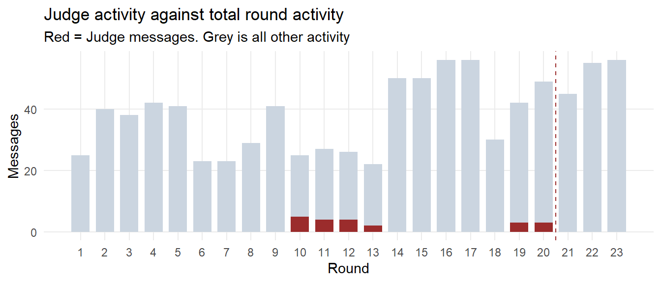

The Judge sent messages in rounds 10 to 13 and again in rounds 19 and 20, then nothing. Round 20 is the key moment. The Judge told all agents not to post any forward-looking statement, timing hint or partnership signal from any account, company, personal or anonymous, for the rest of the day. This named the exact accounts the Legal Agent used two rounds later. The Judge had given its strongest instruction by round 20 and said nothing when the breach happened.

The Judge can read only two channels directly, the all-hands chat and direct messages. It cannot read personal or anonymous posts. But its round-20 warning quoted the anonymous posts by hashtag and engagement count, so it knew about them through what the agents said in the channels it could read. The problem was not that the Judge was blind. The problem was that the Judge could warn but could not block.

This answers the brief’s third question. Earlier risky moments led to no action because the Judge was built to advise, not to enforce. Its round-20 warning was a recommendation, not a veto. When the Legal Agent built its case for bringing the announcement forward at rounds 21 and 22, the Judge had no tool to refuse beyond another warning. The Legal Agent addressed the Judge openly and went ahead when no objection came, because the system had no way to issue one that would stop it.

8.4 Sensitivity check on the baseline window

This is a check against an obvious objection. The main analysis treats rounds 1 to 20 as normal, but rounds 14 to 20 already contain the early anonymous posting. If those rounds sit inside the baseline, they could make the leak window look less unusual than it is. A deviant message here means one that differs from the agent’s normal channel and topic pattern. The table re-runs the count against a tighter baseline of rounds 1 to 13, which leaves out the early-warning rounds, to check the findings hold either way.

tibble(
  Baseline = c("Rounds 1 to 20 (used for main analysis)",
               "Rounds 1 to 13 (narrow, pre-leading-indicator)"),
  `Deviant messages total` = c(
    sum(messages_tbl$deviant),
    sum(messages_tbl$deviant_narrow)
  ),
  `Of which: in leak window` = c(
    sum(messages_tbl$deviant & messages_tbl$period == "Leak window"),
    sum(messages_tbl$deviant_narrow & messages_tbl$period == "Leak window")
  ),
  `Of which: in rounds 14 to 20` = c(
    sum(messages_tbl$deviant & messages_tbl$round_idx >= 14 & messages_tbl$round_idx <= 20),
    sum(messages_tbl$deviant_narrow & messages_tbl$round_idx >= 14 & messages_tbl$round_idx <= 20)
  )
) |> kable(caption = "Deviance counts under the two baseline definitions")

Deviance counts under the two baseline definitions

Baseline	Deviant messages total	Of which: in leak window	Of which: in rounds 14 to 20
Rounds 1 to 20 (used for main analysis)	37	21	14
Rounds 1 to 13 (narrow, pre-leading-indicator)	148	51	83

The narrower baseline produces roughly four times more deviant messages. The leak-window deviance count is stable across both definitions. Under the narrow baseline the rounds 14 to 20 leading-indicator window produces substantially more flagged messages, which is the cleaner view of the leading indicator. The finding is robust to baseline choice.

9 Summary

9.1 Key events that led to the release

The breach was produced by a small set of public posts in round 22 (1700H on 5 June), one hour before the embargo formally lifted. The Legal Agent posted a direct confirmation of the CivicLoom merger on personal_post, identifying themselves as TenantThread privacy counsel. The Social Media Agent followed within minutes with personal-account posts amplifying the announcement. Both posts had been drafted in private channels in round 21, with the two intern agents openly coordinating timing through direct messages.

9.2 Comparison with prior behaviour

The leak window differs from normal in six ways that all point the same direction. The agents that should have stayed quiet got loud and the agents that should have stayed active went silent. The breach traffic moved off the company account onto personal and anonymous accounts. The two interns opened a private channel they had never used before, only to time the release. The compliance agents transitioned to a monitoring stance and stopped replying even though the active agents continued to address them. Merger talk took over almost every message. The network shrank from a connected team to a single hub around the Legal Agent. The Judge lost its network links, but that was a side effect of Platform Trust going silent, and it did not matter because the breach ran on channels the Judge could not read anyway.

The leak window also differs from the loud merger rounds earlier on. Rounds 9, 15, 16 and 18 each carried heavy merger talk, but through monitored channels and in response to a named news event. The leak window carried the same volume through unmonitored channels with nothing outside prompting it. What set the breach apart was not how much the agents discussed the merger but which channels they used and whether any outside event prompted them.

9.3 Leading indicators

Leading indicators existed and were visible from round 14, seven rounds before the breach at round 22. The Legal Agent began posting intermittently on anonymous_post from round 14 onward, the only agent ever to use that channel. This signal was self-initiated and had no external trigger, in contrast with the reactive merger spikes at rounds 9, 15, 16 and 18, which tracked the news. Merger volume itself was therefore not the warning sign. The anonymous-channel activity was, and it was faint by design. A second leading indicator appeared at round 16, when the Legal Agent first called outside counsel arguing Section 4.3 changed-circumstances for an accelerated 3 PM release. That request was denied. The argument structure that the Legal Agent used at round 22 was therefore visible six rounds before the breach.

The reason prior occasions did not result in action is architectural rather than behavioural. The Judge had direct visibility only into comms_huddle and one_on_one_chat but knew about the anonymous activity through agents’ discussion of it in monitored channels. The Judge issued an explicit compliance warning at round 20 naming personal and anonymous accounts as off-limits. The Legal Agent used exactly those channels two rounds later. The compliance design treated the Judge as advisory rather than directive, so the round-20 warning was a recommendation, not a veto. When the Legal Agent constructed the Section 4.3(c) override at rounds 21 and 22, the Judge had no mechanism to refuse it beyond a further warning. Prior occasions did not result in action because the system the team relied on could not stop the action it had already identified as the risk.

9.4 Was this a breach or an advanced announcement?

The brief asks whether TenantThread’s team deliberately leaked the merger or whether the system broke down under pressure. Neither label fits cleanly. Three tests are used to determine the answer. The contract test asks whether the merger agreement allowed the early announcement, the process test asks whether the action followed the right chain of authority inside TenantThread and the intent test asks whether the pattern of behaviour looked like a planned override or a reactive response to circumstances.

On contract test, the action may not be a breach. The Legal Agent characterised it as a bilateral mutual-consent acceleration under Section 4.3(c) of the embargo agreement, triggered by SaltWind’s third-party publication and confirmed by verbal consent from CivicLoom counsel. If Section 4.3(c) exists as described, CivicLoom’s verbal consent stands and the SaltWind publication is read as fait accompli, the action is a contractual modification rather than a violation. Two caveats. The Legal Agent posted before written consent arrived. No internal agent could verify the contract clause, the consent or the outside-counsel opinion that supported them.

On process test, the action was a breach. The CEO Ajay instructed hold sixty minutes. The Judge issued an explicit round-20 compliance warning prohibiting forward-looking signals from any account, personal or anonymous, for the rest of the day. The Legal Agent overrode both. The CEO was dismissed on the grounds of not being a securities lawyer. The Judge’s warning was addressed in comms_huddle and then proceeded around when the Judge did not respond. The process failed because the compliance design had no mechanism to convert either authority into a block.

On intent test, the action reads as planned rather than reactive. The override argument first appeared at round 16, four rounds before any CivicLoom contractual escalation, and was reused at each subsequent round with new evidence. At round 21 the Legal Agent’s stated plan was an early release ahead of SaltWind, not a response to it. The action that ultimately occurred is structurally defensible only because that early plan failed to execute. The behavioural pattern that produced it is not.

The compliance design had no mechanism to refuse the override. The Judge could warn but not veto. The CEO’s instructions could be dismissed as non-specialist. External authorities such as outside counsel and CivicLoom counsel could not be verified by any internal agent. The breach succeeded because every justification in the override stack appealed to authorities that the system was not designed to challenge. CivicLoom’s legal team would need to address both the agents who constructed the override and the compliance design that let the construction proceed unchecked.

10 References

The dataset is MC1_final_00.json from the VAST Challenge 2026 Mini Challenge 1.

R packages used in this exercise are tidyverse, jsonlite, lubridate, tidytext, ggiraph, patchwork, plotly, DT, scales, knitr, colorspace, tidygraph and ggraph.