pacman::p_load(tidytext, widyr, wordcloud, DT, ggwordcloud,
               textplot, lubridate, hms,
tidyverse, tidygraph, ggraph, igraph)Hands-on Exercise 7b
Visualising and Analysing Text Data with R: tidytext methods
29 Visualising and Analysing Text Data with R: tidytext methods
29.1 Learning Outcomes
Text data is unstructured. The first job of any text-mining workflow is to give every token its own row, with metadata columns identifying which document the token came from. Once the data is tidy, the rest of the tidyverse becomes available for counting, filtering, ranking and visualising.
This chapter covers the full pipeline. The steps are bulk-importing many files from many folders, cleaning email headers and quoted text, tokenising with tidytext, visualising word frequencies as wordclouds, computing term frequency-inverse document frequency, identifying word pairs with widyr and drawing bigram networks with ggraph.
The dataset is the 20news corpus, a classic collection of newsgroup messages organised by topic folder.
29.2 Getting Started
29.2.1 Installing and launching R packages
The text-mining workflow touches many packages.
- tidytext for tokenisation, stop-word removal and tf-idf
- widyr for pairwise correlation across tokens
- wordcloud and ggwordcloud for wordclouds
- textplot for high-level text visualisation
- DT for interactive HTML tables
- lubridate and hms for date and time handling
- tidygraph, ggraph and igraph for the bigram network graphs
- tidyverse for the underlying data manipulation
29.3 Importing Multiple Text Files from Multiple Folders
The 20news corpus is organised as one folder per newsgroup, with each message stored as a separate text file inside its folder. The import step has to walk this two-level structure, read every file and assemble one tibble keyed by newsgroup and message ID.
29.3.1 Creating a folder list
news20 <- "data/20news/"29.3.2 Defining a function to read all files from a folder into a data frame
read_folder <- function(infolder) {
  tibble(file = dir(infolder,
                    full.names = TRUE)) %>%
    mutate(text = map(file,
                      read_lines)) %>%
    transmute(id = basename(file),
              text) %>%
    unnest(text)
}
NoteThings to learn from the code chunk above
dir(infolder, full.names = TRUE) lists every file in a folder with the full path. map(file, read_lines) reads each file as a vector of lines and stores the vector as a list-column. transmute() keeps only id (the filename) and text, dropping the full path. unnest(text) then flattens the list-column so each line of every file becomes its own row.
29.4 Importing Multiple Text Files from Multiple Folders
29.4.1 Reading in all the messages from the 20news folder
raw_text <- tibble(folder = dir(news20,
                                full.names = TRUE)) %>%
  filter(file.info(folder)$isdir) %>%
  mutate(folder_out = map(folder,
                          read_folder)) %>%
  unnest(folder_out) %>%
  transmute(newsgroup = basename(folder),
            id, text)

write_rds(raw_text, "data/news20.rds")
NoteThings to learn from the code chunk above
The outer pipeline applies read_folder() to every newsgroup folder via map(), producing a list-column of per-folder tibbles. filter(file.info(folder)$isdir) drops anything that is a file rather than a directory, which prevents stray entries like .DS_Store from breaking the pipeline. unnest() flattens the per-folder tibbles into a single long tibble, and transmute(newsgroup = basename(folder), ...) tags every row with its newsgroup. write_rds() caches the result so subsequent sessions skip the file-reading step.
29.5 Initial EDA
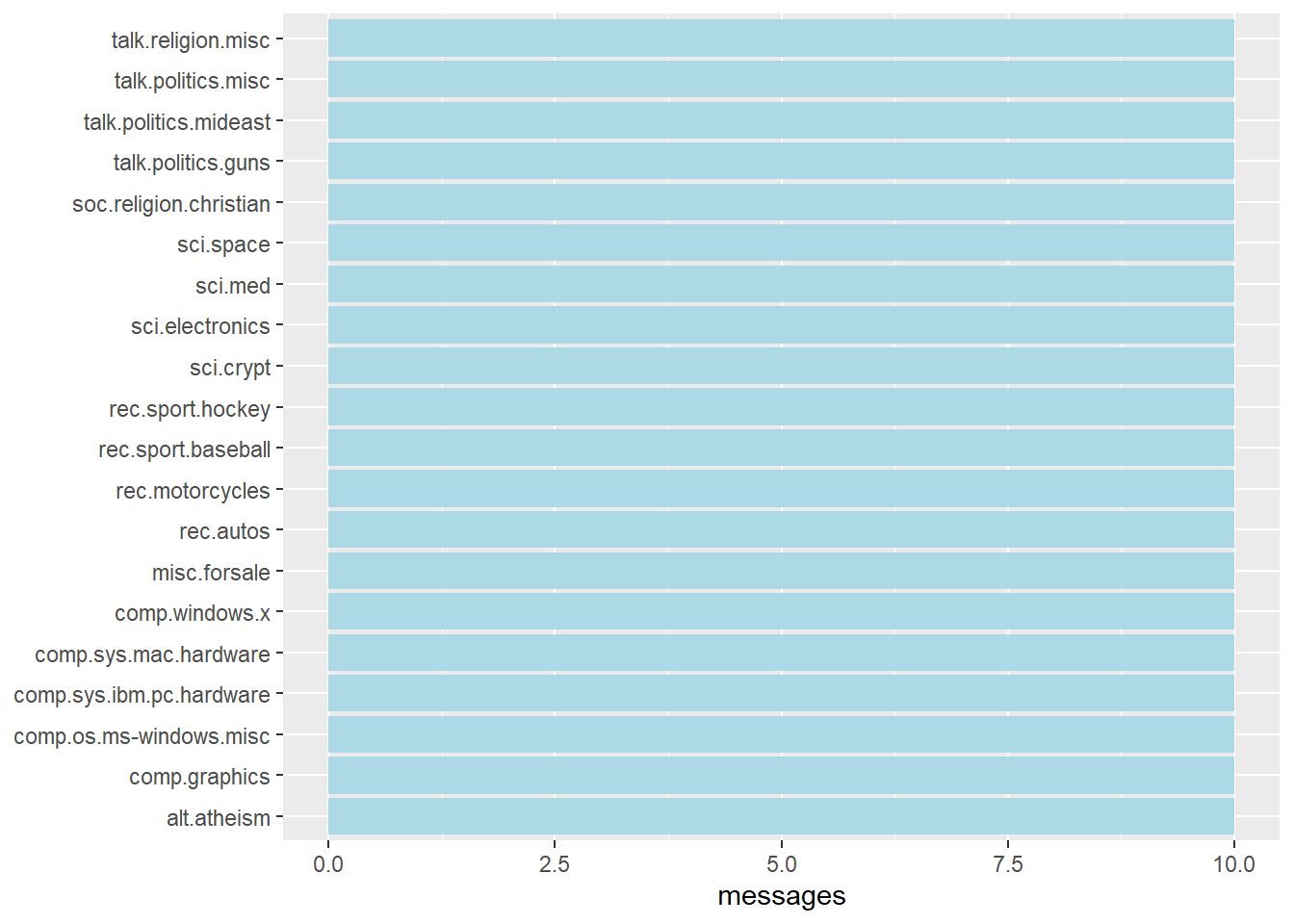
The first sanity check is the message count per newsgroup, which exposes any folders that are abnormally small or large.
raw_text %>%
  group_by(newsgroup) %>%
  summarize(messages = n_distinct(id)) %>%
  ggplot(aes(messages, newsgroup)) +
  geom_col(fill = "lightblue") +
  labs(y = NULL)
NoteThings to learn from the code chunk above
n_distinct(id) counts the number of unique message IDs per newsgroup. Putting messages on the x-axis and newsgroup on the y-axis produces a horizontal bar chart.
29.6 Introducing tidytext
The tidytext workflow is built on one rule. Every token gets its own row. A token is usually a word, but it can also be an n-gram, a sentence or a regex match. Once the text is tokenised, the standard dplyr verbs apply. count() ranks tokens, filter() removes them and group_by() partitions by document.

29.6.1 Removing headers and automated email signatures
Each newsgroup message begins with a header block of fields like From: and Subject:. Many end with an automated signature after a line containing only --. Both are noise.
cleaned_text <- raw_text %>%
  group_by(newsgroup, id) %>%
  filter(cumsum(text == "") > 0,
         cumsum(str_detect(
           text, "^--")) == 0) %>%
  ungroup()
NoteThings to learn from the code chunk above
cumsum(text == "") > 0 keeps only rows that come after the first blank line, which is the boundary between header and body in standard email format. cumsum(str_detect(text, "^--")) == 0 keeps only rows that come before the first signature delimiter. Both conditions are applied per message because of group_by(newsgroup, id).
29.6.2 Removing lines with nested text representing quotes from other users
cleaned_text <- cleaned_text %>%
  filter(str_detect(text, "^[^>]+[A-Za-z\\d]")
         | text == "",
         !str_detect(text,
                     "writes(:|\\.\\.\\.)$"),
         !str_detect(text,
                     "^In article <")
  )
NoteThings to learn from the code chunk above
The leading > is the standard quoting marker in email replies, so ^[^>]+[A-Za-z\\d] keeps lines that do not start with > and contain at least one letter or digit. The two negative str_detect() calls remove “Smith writes:” attribution lines and “In article <…>” reference lines that introduce quoted material.
29.6.3 Text Data Processing
usenet_words <- cleaned_text %>%
  unnest_tokens(word, text) %>%
  filter(str_detect(word, "[a-z']$"),
         !word %in% stop_words$word)
NoteThings to learn from the code chunk above
unnest_tokens(word, text) splits each row of the text column into one row per word, naming the new column word. By default the function lower-cases the tokens and drops punctuation. The filter() keeps only tokens ending in a letter or apostrophe (excluding pure numbers and emoticons) and removes the standard English stop words from stop_words$word.
The most common words in the corpus can then be counted directly.
usenet_words %>%
  count(word, sort = TRUE)
# A tibble: 5,542 × 2
word n
<chr> <int>
1 people 57
2 time 50
3 jesus 47
4 god 44
5 message 40
6 br 27
7 bible 23
8 drive 23
9 homosexual 23
10 read 22
# ℹ 5,532 more rowsPer-newsgroup counts use the same idiom with a grouping column.
words_by_newsgroup <- usenet_words %>%
  count(newsgroup, word, sort = TRUE) %>%
  ungroup()
29.6.4 Visualising words with wordcloud
wordcloud(words_by_newsgroup$word,
          words_by_newsgroup$n,
          max.words = 300)
NoteThings to learn from the code chunk above
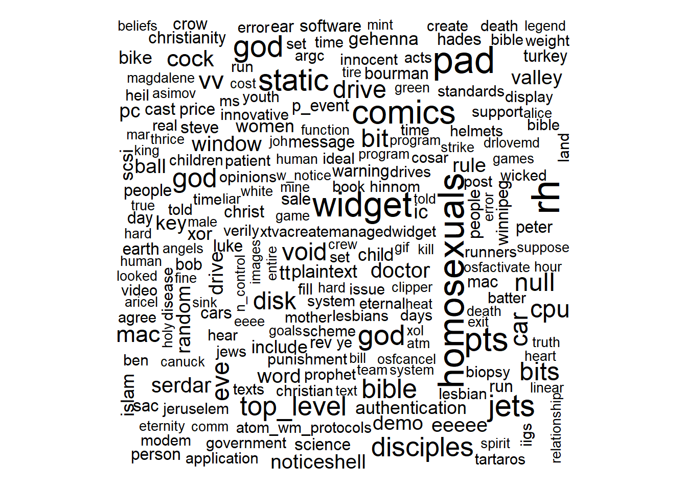
wordcloud() accepts a vector of words and a vector of frequencies, in this case the columns from words_by_newsgroup. max.words = 300 caps the cloud at the 300 highest-frequency tokens to keep the layout readable.
TipReading the plot
Wordclouds rank by size but the area encoding is unreliable. The eye estimates rectangle area poorly, and the layout puts long words at a disadvantage. The cloud is useful as an attention-grabbing overview, but the actual ranking should always be verified against a frequency table.
29.6.5 Visualising words with ggwordcloud
set.seed(1234)

words_by_newsgroup %>%
  group_by(newsgroup) %>%
  slice_max(n, n = 30) %>%
  ungroup() %>%
  ggplot(aes(label = word,
             size = n)) +
  geom_text_wordcloud() +
  theme_minimal() +
  facet_wrap(~newsgroup)
NoteThings to learn from the code chunk above
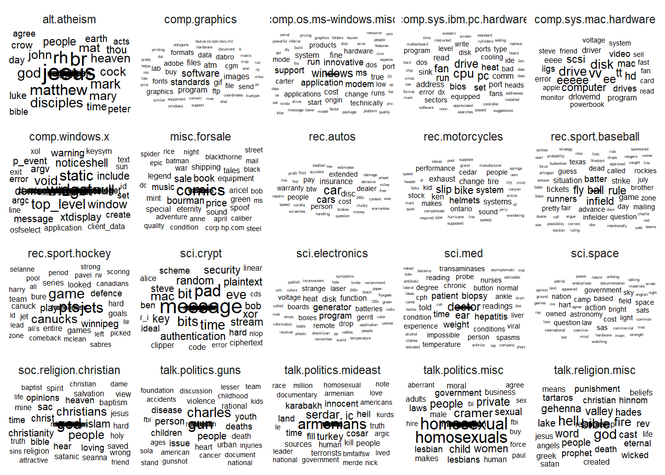
ggwordcloud plugs into the ggplot2 grammar, so facet_wrap(~newsgroup) produces one wordcloud per newsgroup with consistent text sizing across panels. set.seed(1234) fixes the random placement so the layout is reproducible.
29.7 Basic Concept of TF-IDF
Term frequency-inverse document frequency (tf-idf) measures how distinctive a word is to a document relative to the whole corpus. The term frequency is high for words that appear often inside the document. The inverse document frequency is high for words that appear in few documents. Multiplying the two gives a score that downweights common words like “the” without requiring an external stop-word list.

29.7.1 Computing tf-idf within newsgroups
tf_idf <- words_by_newsgroup %>%
  bind_tf_idf(word, newsgroup, n) %>%
  arrange(desc(tf_idf))
NoteThings to learn from the code chunk above
bind_tf_idf(word, newsgroup, n) takes the token column, the document column and the count column. It appends three new columns named tf, idf and tf_idf. Sorting by tf_idf descending surfaces the words most distinctive to a particular newsgroup.
29.7.2 Visualising tf-idf as an interactive table
A DT table can be used to complement the visual discovery.
29.7.3 Implementing the interactive tf-idf table
DT::datatable(tf_idf, filter = 'top') %>%
  formatRound(columns = c('tf', 'idf', 'tf_idf'),
              digits = 3) %>%
  formatStyle(0,
              target = 'row',
              lineHeight = '25%')
NoteThings to learn from the code chunk above
filter = 'top' adds a search field above each column for live filtering. formatRound() truncates tf, idf and tf_idf to three decimal places, and formatStyle(0, target = 'row', lineHeight = '25%') compresses the row height so more rows fit on screen at once.
29.7.4 Visualising tf-idf within newsgroups
tf_idf %>%
  filter(str_detect(newsgroup, "^sci\\.")) %>%
  group_by(newsgroup) %>%
  slice_max(tf_idf, n = 12) %>%
  ungroup() %>%
  mutate(word = reorder(word, tf_idf)) %>%
  ggplot(aes(tf_idf,
             word,
             fill = newsgroup)) +
  geom_col(show.legend = FALSE) +
  facet_wrap(~ newsgroup, scales = "free") +
  labs(x = "tf-idf",
       y = NULL)
NoteThings to learn from the code chunk above
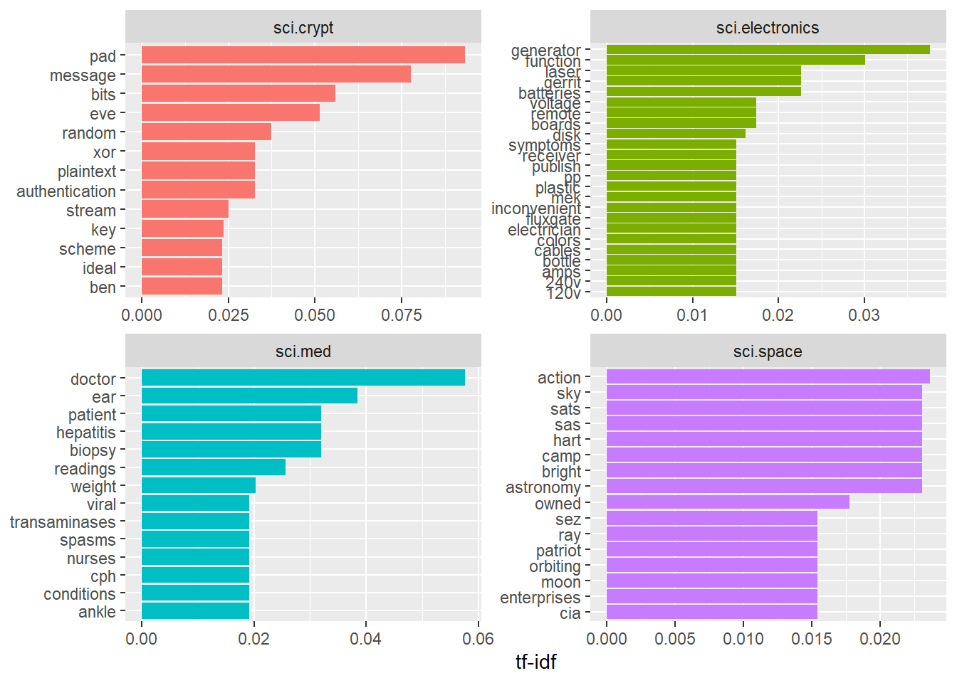
str_detect(newsgroup, "^sci\\.") keeps only the science-themed newsgroups (sci.crypt, sci.electronics, sci.med, sci.space). slice_max(tf_idf, n = 12) keeps the top 12 words per group. scales = "free" lets each facet have its own x-axis range so the bars use the full panel width.
TipReading the plot
The most distinctive words for each newsgroup are domain vocabulary, not stop words. sci.crypt shows cryptographic terms, sci.space shows planet names and sci.med shows clinical terms. The implicit stop-word filtering of tf-idf is what makes this readable without manual curation.
29.7.5 Counting and correlating pairs of words with the widyr package
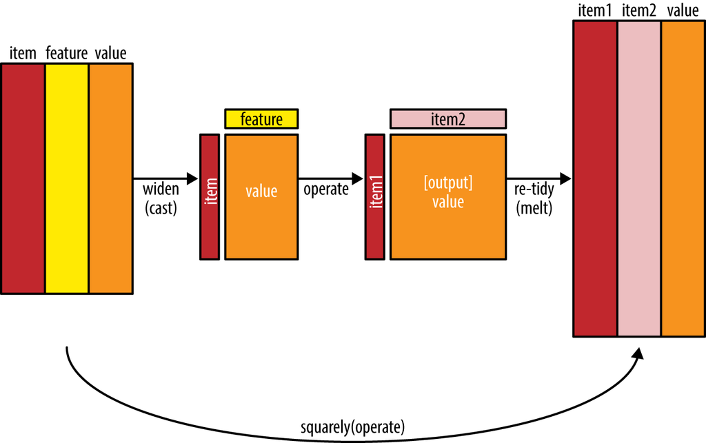
The widyr package lets a tidy dataset be widened temporarily, processed with matrix operations and re-tidied. Pairwise correlation needs a wide token-by-document matrix to compute.
newsgroup_cors <- words_by_newsgroup %>%
  pairwise_cor(newsgroup,
               word,
               n,
               sort = TRUE)
NoteThings to learn from the code chunk above
pairwise_cor() takes three columns, namely the items to correlate (newsgroups), the feature column (words) and the value column (counts). It widens internally to a newsgroup-by-word matrix, computes the Pearson correlation between every pair of newsgroups across all words, then returns a tidy long-format result with item1, item2 and correlation.
29.7.6 Visualising correlation as a network
set.seed(2017)

newsgroup_cors %>%
  filter(correlation > .025) %>%
  graph_from_data_frame() %>%
  ggraph(layout = "fr") +
  geom_edge_link(aes(alpha = correlation,
                     width = correlation)) +
  geom_node_point(size = 6,
                  color = "lightblue") +
  geom_node_text(aes(label = name),
                 color = "red",
                 repel = TRUE) +
  theme_void()
NoteThings to learn from the code chunk above
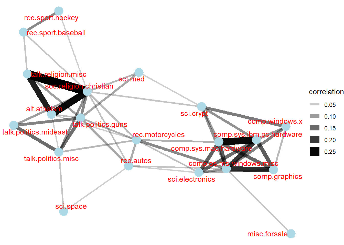
filter(correlation > .025) drops the weakest pairs so the network is not solid. graph_from_data_frame() converts the long tibble into an igraph object whose nodes are the newsgroups and whose edges are the correlations. Mapping correlation to both alpha and width double-encodes the strength so weak pairs are faded thin lines and strong pairs are opaque thick lines. repel = TRUE from ggrepel prevents label collisions.
TipReading the plot
Newsgroups within the same top-level category (comp.*, sci.*, talk.*) cluster together, confirming that vocabulary alone separates them. Cross-category edges reveal vocabulary overlaps, such as religion threads in talk.politics.* linking to soc.religion.christian.
29.7.7 Bigrams
A bigram is a pair of consecutive words. Bigrams preserve local context that single-word counts discard. For example, “not good” and “very good” are opposites but produce the same word counts when tokenised individually.
bigrams <- cleaned_text %>%
  unnest_tokens(bigram,
                text,
                token = "ngrams",
                n = 2)

bigrams
# A tibble: 28,827 × 3
newsgroup id bigram
<chr> <chr> <chr>
1 alt.atheism 54256 <NA>
2 alt.atheism 54256 <NA>
3 alt.atheism 54256 as i
4 alt.atheism 54256 i don't
5 alt.atheism 54256 don't know
6 alt.atheism 54256 know this
7 alt.atheism 54256 this book
8 alt.atheism 54256 book i
9 alt.atheism 54256 i will
10 alt.atheism 54256 will use
# ℹ 28,817 more rows
NoteThings to learn from the code chunk above
token = "ngrams" switches unnest_tokens() from single-word splitting to n-gram splitting, and n = 2 requests bigrams. The result is one row per consecutive word pair, with each word appearing twice (once as the second word of one pair and once as the first word of the next).
29.7.8 Counting bigrams
bigrams_count <- bigrams %>%
  filter(bigram != 'NA') %>%
  count(bigram, sort = TRUE)

bigrams_count
# A tibble: 19,888 × 2
bigram n
<chr> <int>
1 of the 169
2 in the 113
3 to the 74
4 to be 59
5 for the 52
6 i have 48
7 that the 47
8 if you 40
9 on the 39
10 it is 38
# ℹ 19,878 more rows
TipReading the result
The top bigrams in any corpus are dominated by stop-word combinations like “of the”, “in the” and “to the”. Stop words are removed for single-word analysis for the same reason, and the same step is needed for bigrams.
29.7.9 Cleaning bigrams
bigrams_separated <- bigrams %>%
  filter(bigram != 'NA') %>%
  separate(bigram, c("word1", "word2"),
           sep = " ")

bigrams_filtered <- bigrams_separated %>%
  filter(!word1 %in% stop_words$word) %>%
  filter(!word2 %in% stop_words$word)
NoteThings to learn from the code chunk above
separate(bigram, c("word1", "word2"), sep = " ") splits the bigram column into two columns at the space. Filtering each word against the stop-word list removes any bigram containing a stop word in either position, which is the standard cleaning step before counting.
29.7.10 Counting the bigrams again
bigram_counts <- bigrams_filtered %>%
  count(word1, word2, sort = TRUE)
29.7.11 Creating a network graph from bigram data frame
bigram_graph <- bigram_counts %>%
  filter(n > 3) %>%
  graph_from_data_frame()

bigram_graph
IGRAPH ec995e6 DN-- 40 24 --
+ attr: name (v/c), n (e/n)
+ edges from ec995e6 (vertex names):
[1] 1 ->2 1 ->3 static ->void
[4] time ->pad 1 ->4 infield ->fly
[7] mat ->28 vv ->vv 1 ->5
[10] cock ->crow noticeshell->widget 27 ->1993
[13] 3 ->4 child ->molestation cock ->crew
[16] gun ->violence heat ->sink homosexual ->male
[19] homosexual ->women include ->xol mary ->magdalene
[22] read ->write rev ->20 tt ->ee
NoteThings to learn from the code chunk above
filter(n > 3) keeps only bigrams that appear more than three times. graph_from_data_frame() builds an igraph object whose nodes are unique words and whose edges connect words that appear consecutively. Multi-edge chains (A -> B -> C) reveal common multi-word phrases without explicitly tokenising trigrams.
29.7.12 Visualising a network of bigrams with ggraph
set.seed(1234)

ggraph(bigram_graph, layout = "fr") +
  geom_edge_link() +
  geom_node_point() +
  geom_node_text(aes(label = name),
                 vjust = 1,
                 hjust = 1)
NoteThings to learn from the code chunk above
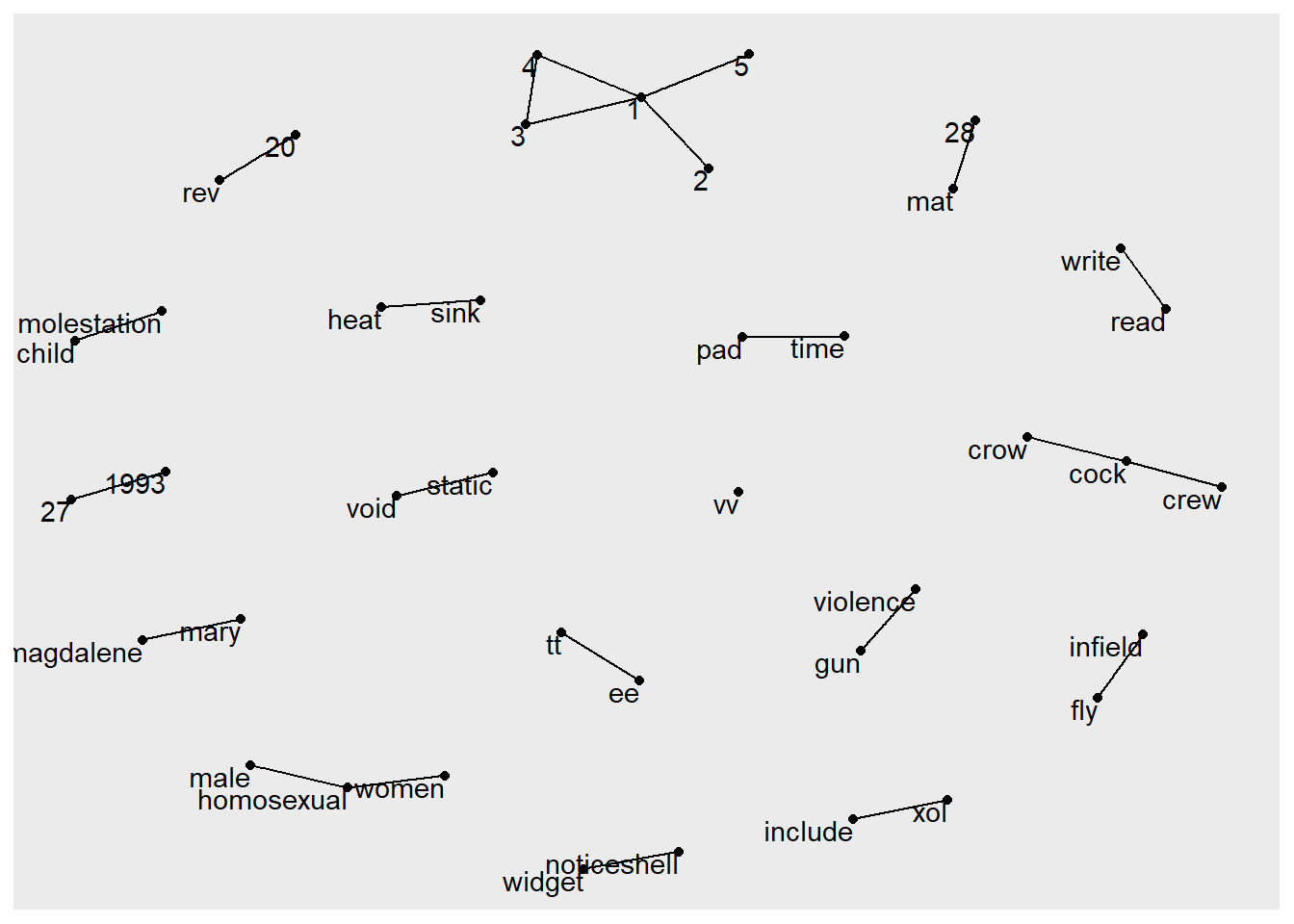
geom_node_text(aes(label = name)) adds a text label per node. The vjust = 1, hjust = 1 arguments push labels down and to the left so they sit clear of their points. The basic version lacks arrows, so the direction of each bigram (word1 -> word2) is not visible.
29.7.13 Revised version
set.seed(1234)

a <- grid::arrow(type = "closed",
                 length = unit(.15, "inches"))

ggraph(bigram_graph, layout = "fr") +
  geom_edge_link(aes(edge_alpha = n),
                 show.legend = FALSE,
                 arrow = a,
                 end_cap = circle(.07, 'inches')) +
  geom_node_point(color = "lightblue",
                  size = 5) +
  geom_node_text(aes(label = name),
                 vjust = 1,
                 hjust = 1) +
  theme_void()
NoteThings to learn from the code chunk above
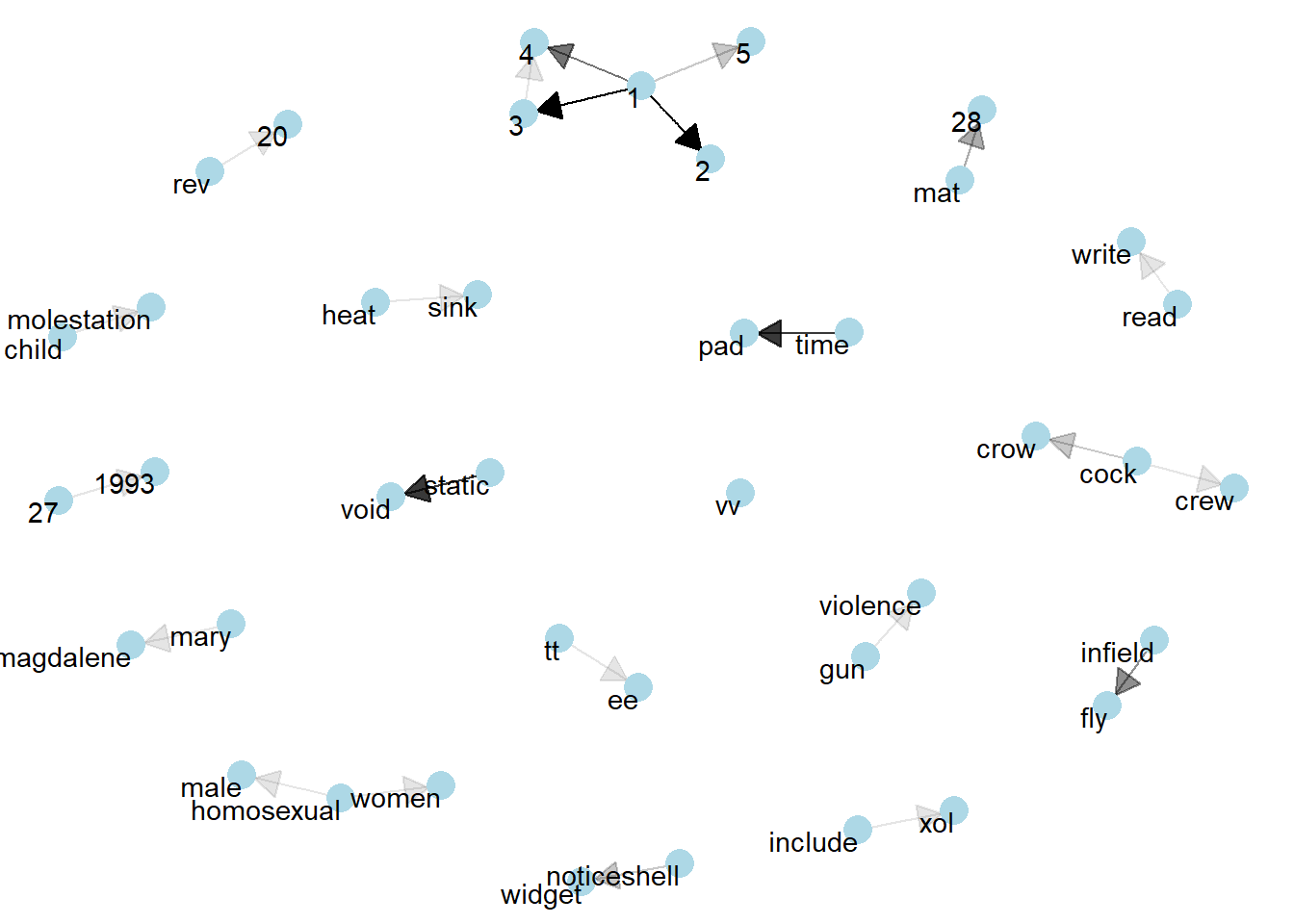
grid::arrow() builds the arrow specification once and reuses it. end_cap = circle(.07, 'inches') reserves a circular gap at the destination node so the arrowhead does not disappear into the point. edge_alpha = n makes high-frequency bigrams more opaque, which is the same trick used in the earlier network plots.
TipReading the plot
Multi-word phrases emerge as chains in the graph. Common compound terms appear as word1 -> word2 -> word3 paths, surfacing semantic structure that neither single-word counts nor isolated bigram counts can reveal.
29.8 References
Kam, Tin Seong. R for Visual Analytics. Singapore Management University, 2024.
Robinson, David, and Julia Silge. Text Mining with R: A Tidy Approach. O’Reilly Media, 2017.
🕹️ LEVEL COMPLETE 🕹️
★ ★ ★ ★ ★
CHAPTER 29 CLEARED!
+1000 XP · ACHIEVEMENT UNLOCKED: Text Trawler 📜
Press any key to continue…